Signal conversion using PCM and PWM
In this example, let's compare pulse-code modulation (PCM) and pulse-width modulation (PWM) in the Engee model. Let's measure the quantization and encoding errors, estimate the filter delay, and check the dependence of the average PWM value on the input signal.
Sampling and quantization
When sampling, we take samples . To restore a band-limited signal, the sampling frequency must exceed twice the upper frequency of the spectrum.
The quantizer rounds the samples in increments :
For a uniformly distributed error, its RMS value is estimated as .
Encoding and decoding
For bits and range the step is equal to . The signed code takes values from before , and the decoder multiplies the code by . Upper recoverable level — .
The ratio of signal power to quantization error power:
Pulse width modulation
The PWM signal switches between 0 and 1. Its average value over the period is equal to the fill factor:
With a discrete step the filling changes incrementally .
Description of the model
Model pcm_pwm_analysis shown in the picture below.
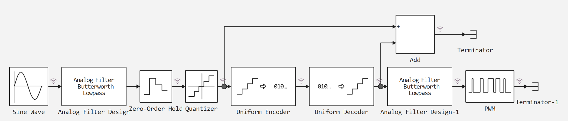
The model contains PCM and PWM branches. Filtering, sampling, quantization, encoding, and decoding are performed sequentially in PCM.
[PIPE] Error signal [PIPE] What is being compared [PIPE]
[PIPE]---[PIPE]---[PIPE]
[PIPE] quant_error [PIPE] Input and output of the quantizer [PIPE]
[PIPE] pcm_error [PIPE] Quantized and decoded signals [PIPE]
[PIPE] total_error [PIPE] Quantizer input and decoded signal [PIPE]
We evaluate the delay of filters separately from coding errors.
Let's prepare the analysis functions.
using Main: engee, plot, plot!, histogram, hline!, savefig, Animation, frame, gif
using Statistics
Let's set the model parameters and calculate the quantization step and the expected SQNR.
# Parameters of the pcm_pwm_analysis model blocks
A      = 0.5         # The amplitude of the Sine Wave
Ω      = 1.0         # Sine Wave frequency, rad/s
ωc     = 30.0        # cutoff frequency of Analog Filter Design filters, rad/s
N      = 8           # filter order
Ts     = 0.01        # Sample Time of the Zero-Order Hold block, with
q_set  = 0.0078125   # Quantization interval of the Quantizer block
V      = 1.0         # The peak of the Uniform Encoder and Uniform Decoder blocks
B      = 8           # Bits of the Uniform Encoder and Uniform Decoder blocks
T_pwm  = 0.05        # Period of the PWM block, with
Ts_pwm = 0.001       # Sample Time of the PWM block, with

q = 2V / 2^B
sqnr_theory = 10 * log10((A^2 / 2) / (q^2 / 12))

println("Шаг кодера q = 2V/2^B: ", q, "; matches the Quantizer interval: ", q == q_set)
println("Предел ошибки квантования q/2: ", q / 2)
println("СКЗ ошибки при равномерном распределении q/√12: ", round(q / sqrt(12), sigdigits = 4))
println("Level 1.0 code without saturation: ", round(Int, 1.0 / q), "; the largest code: ", 2^(B - 1) - 1)
println("SQNR estimation for a sine wave of amplitude ", A, ": ", round(sqnr_theory, digits = 1), " dB")
println("Шаг коэффициента заполнения PWM T_pwm/T: ", Ts_pwm / T_pwm)
The maximum signed code is 127, so we can't accurately represent the 1.0 level. For the signal amplitude used, the expected SQNR is about 44 dB.
The transfer function of the Butterworth filter is obtained from its poles:
Let's estimate the gain and delay at the signal frequency by modulus and phase .
# Poles and frequency response of an analog Butterworth filter
poles = [ωc * exp(im * π * (2k + N - 1) / (2N)) for k in 1:N]
H(s) = prod(-p / (s - p) for p in poles)

H_sig = H(im * Ω)
τ_filter = -angle(H_sig) / Ω

println("Module |H(jΩ)| at the signal frequency: ", round(abs(H_sig), digits = 6))
println("Phase delay of a single filter: ", round(τ_filter, digits = 4), " with")
println("Group delay at zero frequency: ", round(1 / (ωc * sin(π / (2N))), digits = 4), " with")
One filter gives a delay of about 0.17 s at a gain close to unity. Two consecutive filters roughly double the delay.
Download the model from the example folder and run the calculation.
model_name = "pcm_pwm_analysis"
model_file = joinpath(@__DIR__, model_name * ".engee")

model = engee.load(model_file; force = true)
results = engee.run(model);
We will receive the recorded signals and close the model.
x_sine  = collect(results["Sine Wave.1"])
x_zoh   = collect(results["Zero-Order Hold.1"])
x_quant = collect(results["Quantizer.1"])
x_code  = collect(results["Uniform Encoder.1"])
x_dec   = collect(results["Uniform Decoder.1"])
x_add   = collect(results["Add.1"])
x_duty  = collect(results["Analog Filter Design-1.1"])
x_pwm   = collect(results["PWM.1"])

engee.close(model_name; force = true)

signals = ["Sine Wave" => x_sine, "Zero-Order Hold" => x_zoh, "Quantizer" => x_quant,
           "Uniform Encoder" => x_code, "Uniform Decoder" => x_dec, "Add" => x_add,
           "Analog Filter Design-1" => x_duty, "PWM" => x_pwm]

for (name, s) in signals
    println(rpad(name, 24), length(s.time), " points, t from ", first(s.time), " before ", last(s.time),
            " с, шаг ≈ ", round(median(diff(s.time)), sigdigits = 3), " с, тип ", eltype(s.value))
end
The signals are recorded on different time grids. Let's bring them to a common grid for comparison.
The hold_at function selects the last countdown preceding the specified time point. We use it to compare script errors with the outputs of the model blocks.
function hold_at(s, t)
    idx = searchsortedlast.(Ref(s.time), t .+ 1e-6)
    return s.value[clamp.(idx, 1, length(s.time))]
end

rms(x) = sqrt(mean(abs2, x))

t_k = collect(0:Ts:last(x_zoh.time))

u_k   = hold_at(x_zoh, t_k)          # Quantizer input (Zero-Order Hold output)
y_k   = hold_at(x_quant, t_k)        # Quantizer output
c_k   = Int.(hold_at(x_code, t_k))   # Uniform Encoder Codes
d_k   = hold_at(x_dec, t_k)          # Uniform Decoder output
add_k = hold_at(x_add, t_k)          # Add output

quant_error = y_k .- u_k             # Quantizer − Zero-Order Hold
pcm_error   = y_k .- d_k             # Quantizer − Uniform Decoder
total_error = d_k .- u_k             # Uniform Decoder − Zero-Order Hold

println("Sampling moments: ", length(t_k))
println("The largest discrepancy between pcm_error and Add output: ", maximum(abs.(pcm_error .- add_k)))
The calculated PCM error coincides with the signal of the corresponding Add block.
Quantization error
Let's check the limits of the quantization error and its RMS value.
println("Quantizer Quantization Error − Zero-Order Hold")
println("  the largest module: ", round(maximum(abs.(quant_error)), sigdigits = 5), " (предел q/2 = ", q / 2, ")")
println("  SKZ: ", round(rms(quant_error), sigdigits = 5), " (оценка q/√12 = ", round(q / sqrt(12), sigdigits = 5), ")")
println("  average: ", round(mean(quant_error), sigdigits = 3))
The error does not exceed ±q/2. Let's compare its distribution with the estimate of q/√12.
histogram(quant_error ./ q;
    bins = range(-0.5, 0.5; length = 21),
    normalize = :pdf,
    label = "quant_error / q",
    xlabel = "Error in fractions of a step q",
    ylabel = "Density",
    title = "Distribution of the quantization error",
    size = (900, 400))
hline!([1.0]; label = "Uniform distribution", linestyle = :dash, linewidth = 2)
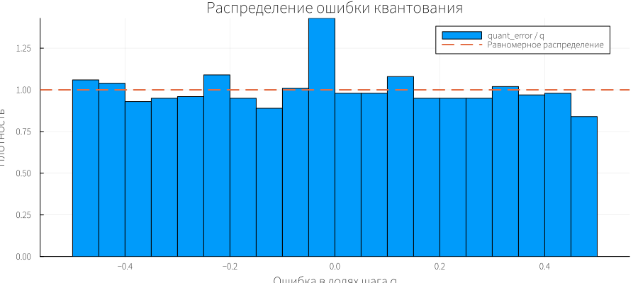
The histogram does not have to be uniform: in 20 seconds of simulation, the slow input signal passes through only a few periods.
We'll find the encoding error and check what's going on at the top level 1.0.
nz = findall(abs.(pcm_error) .> q / 2)
share = length(nz) / length(t_k)

println("Quantizer codec error − Uniform Decoder (Add output)")
println("  the largest module: ", maximum(abs.(pcm_error)))
println("  SKZ: ", round(rms(pcm_error), sigdigits = 5), "; q·√(fraction of non-zero values): ", round(q * sqrt(share), sigdigits = 5))
println("  non-zero counts: ", length(nz), " from ", length(t_k), " (", round(100share, digits = 2), " %)")
println("  Quantizer values in these counts: ", unique(y_k[nz]))
println("  Uniform Encoder codes in these counts: ", unique(c_k[nz]))
println("  counts with the Quantizer 1.0 level: ", count(==(1.0), y_k))
println("  range of codes per calculation: from ", minimum(c_k), " before ", maximum(c_k))
The 127 code is restored as 1−q. Therefore, an error of magnitude q appears at the top of the signal.
Consider the area near the vertex and mark the error boundaries.
i0 = isempty(nz) ? argmax(y_k) : first(nz)
win = abs.(t_k .- t_k[i0]) .<= 0.3

plot(t_k[win], u_k[win];
    seriestype = :steppost, label = "Zero-Order Hold", linewidth = 2,
    xlabel = "Time, from", ylabel = "Level",
    title = "Samples at the top of the sine wave",
    legend = :outertopright, size = (1000, 450))
plot!(t_k[win], y_k[win]; seriestype = :steppost, label = "Quantizer", linewidth = 2)
plot!(t_k[win], d_k[win]; seriestype = :steppost, label = "Uniform Decoder", linewidth = 2, linestyle = :dash)
hline!([1.0, 1 - q]; label = "Levels 1.0 and 1 − q", color = :gray, linestyle = :dot)
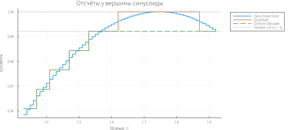
Up to level 1.0, the outputs of the quantizer and decoder match. At the top, the decoder is limited to the 127/128 level.
Let's compare the quantization and encoding errors and their total result.
plot(t_k, quant_error;
    label = "quant_error: Quantizer − Zero-Order Hold", linewidth = 1,
    xlabel = "Time, from", ylabel = "Mistake",
    title = "Errors between model points",
    legend = :outertopright, size = (1100, 450))
plot!(t_k, pcm_error; label = "pcm_error: Quantizer − Uniform Decoder", linewidth = 1.5)
plot!(t_k, total_error; label = "total_error: Uniform Decoder − Zero-Order Hold", linewidth = 1, alpha = 0.6)
hline!([q / 2, -q / 2]; label = "±q/2", color = :gray, linestyle = :dash)
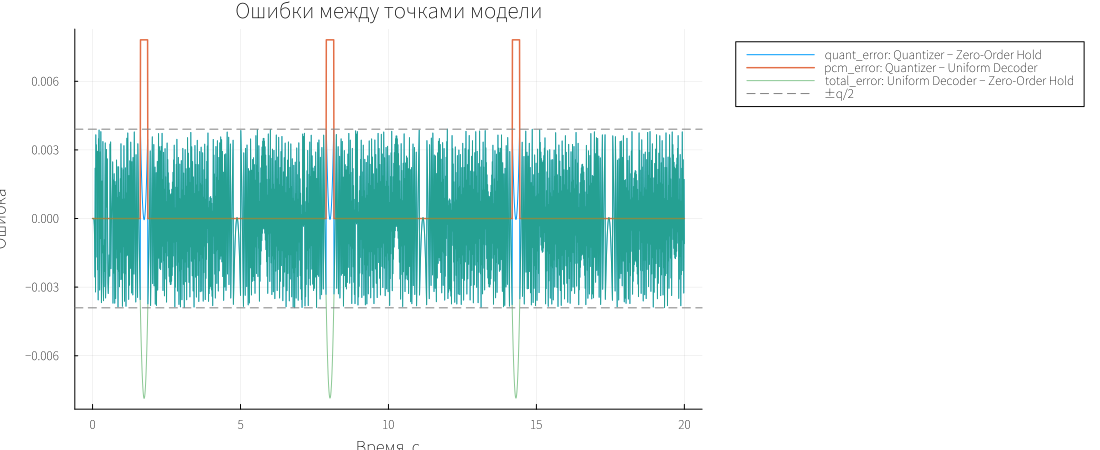
The quantization error is limited to ±q/2, and the PCM error appears at the vertices. Therefore, the total error may exceed the error limits of a single quantizer.
Let's calculate the SQNR after the first two seconds, excluding the initial transient.
steady = t_k .>= 2.0
p_signal = var(u_k[steady])

sqnr_quant = 10 * log10(p_signal / mean(abs2, quant_error[steady]))
sqnr_total = 10 * log10(p_signal / mean(abs2, total_error[steady]))

println("SQNR by quantization error: ", round(sqnr_quant, digits = 1), " dB")
println("SQNR for the final error:    ", round(sqnr_total, digits = 1), " dB")
println("Theoretical assessment:        ", round(sqnr_theory, digits = 1), " dB")
The upper level restriction adds error and reduces the SQNR of the recovered signal.
Let's find the delay at which the RMS difference of the signals is minimal. Let's check the range 0-0.5 s in 1 ms increments.
τ_grid = 0:0.001:0.5
lag_rms = [rms(d_k[steady] .- hold_at(x_sine, t_k[steady] .- τ)) for τ in τ_grid]
τ_est = τ_grid[argmin(lag_rms)]

println("Data delay: ", τ_est, " c; calculation for a single filter: ", round(τ_filter, digits = 4), " with")
println("SKZ of the difference without a shift: ", round(rms(d_k[steady] .- hold_at(x_sine, t_k[steady])), sigdigits = 4))
println("SKZ differences with a shift: ", round(minimum(lag_rms), sigdigits = 4))
Let's compare the found delay with the calculation of the filter phase and apply the signals taking into account the shift.
plot(t_k, hold_at(x_sine, t_k);
    label = "Sine Wave", linewidth = 2,
    xlabel = "Time, from", ylabel = "The amplitude",
    title = "Generator output and PCM decoder output",
    legend = :outertopright, size = (1100, 450))
plot!(t_k, d_k; label = "Uniform Decoder", linewidth = 2, linestyle = :dash)
plot!(t_k, hold_at(x_sine, t_k .- τ_est); label = "Sine Wave, a shift of τ", linewidth = 1.5, linestyle = :dot)
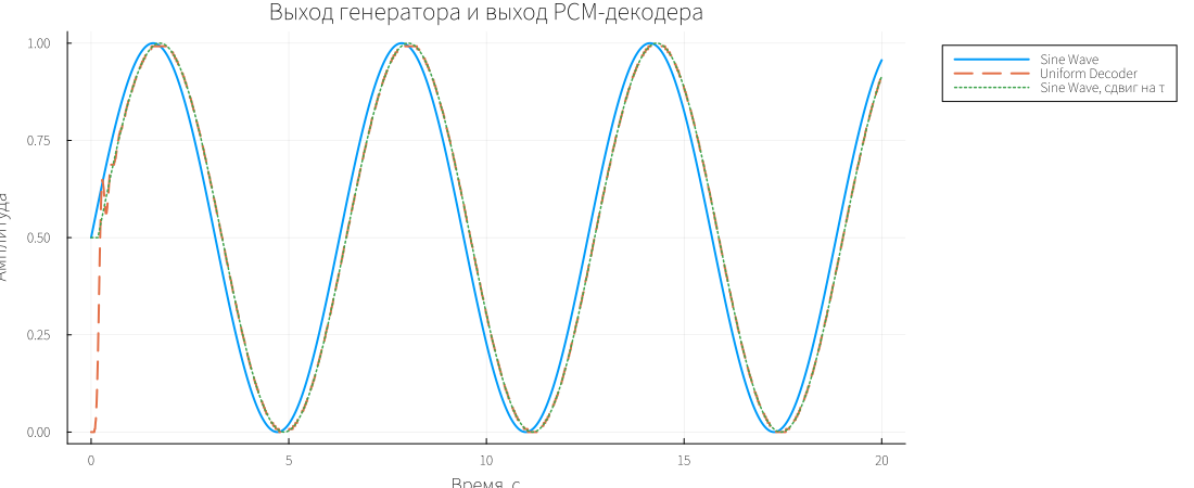
After the delay compensation, the signals almost match. The main difference before the shift is related to filtering.
Let's see what codes the model uses.
plot(t_k, c_k;
    seriestype = :steppost, label = "Uniform Encoder", linewidth = 1.5,
    xlabel = "Time, from", ylabel = "Code",
    title = "Codes at the output of the PCM encoder",
    legend = :outertopright, size = (1100, 400))
hline!([2^(B - 1) - 1]; label = "The largest code is 127", color = :gray, linestyle = :dash)
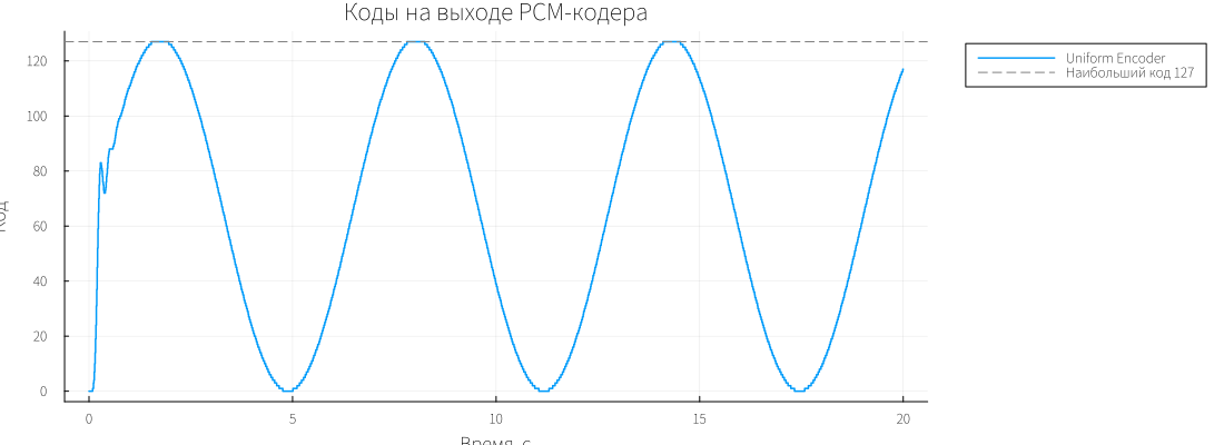
Codes from 0 to 127 are used for this input signal. The upper bound limits the vertex recovery.
For PWM, we use a 1 ms grid and a period of 0.05 s. Let's calculate the average value for each period; the filling step is 0.02.
n_per = round(Int, T_pwm / Ts_pwm)
t_all = collect(0:Ts_pwm:last(x_pwm.time) - Ts_pwm)
n_periods = length(t_all) ÷ n_per
t_p = t_all[1:n_per * n_periods]     # only whole periods

pwm_p  = hold_at(x_pwm,  t_p)
duty_p = hold_at(x_duty, t_p)

pwm_avg  = vec(mean(reshape(pwm_p,  n_per, n_periods); dims = 1))
duty_avg = vec(mean(reshape(duty_p, n_per, n_periods); dims = 1))
t_avg    = T_pwm .* (0:n_periods - 1)
pwm_dev  = pwm_avg .- duty_avg

println("PWM output Values: ", first(sort(unique(pwm_p)), 5))
println("Counts for the period: ", n_per, "; periods: ", n_periods)
println("Average PWM input per calculation: ", round(mean(duty_p), digits = 5))
println("Average PWM output per calculation: ", round(mean(pwm_p), digits = 5))
println("Difference of averages for the period: average ", round(mean(pwm_dev), digits = 4),
        ", от ", round(minimum(pwm_dev), digits = 4), " до ", round(maximum(pwm_dev), digits = 4))
println("Средние выхода за период кратны 1/", n_per, ": ",
        all(isapprox.(pwm_avg .* n_per, round.(pwm_avg .* n_per); atol = 1e-9)))
The average PWM value follows the input. The deviations are related to the discrete step of filling and changing the input during the period.
Let's show the pulses in the first 0.5 seconds of simulation.
win_p = t_p .<= 0.5

plot(t_p[win_p], pwm_p[win_p];
    seriestype = :steppost, label = "PWM output", linewidth = 1.2,
    ylims = (-0.05, 1.05),
    xlabel = "Time, from", ylabel = "Level",
    title = "The PWM output and the control signal at its input",
    legend = :outertopright, size = (1100, 450))
plot!(t_p[win_p], duty_p[win_p]; label = "PWM input", linewidth = 2)
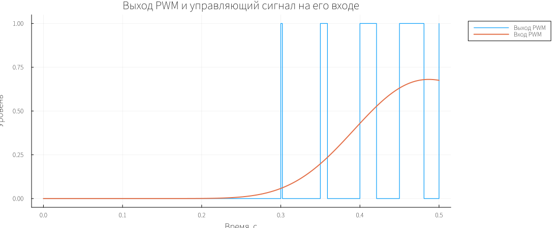
As the input signal grows, the pulse width increases.
Let's compare the average PWM with the input and plot their difference.
p_avg = plot(t_avg, duty_avg;
    label = "PWM input, average over the period", linewidth = 2,
    ylabel = "Level", title = "Average values for the PWM period",
    legend = :outertopright)
plot!(p_avg, t_avg, pwm_avg; seriestype = :steppost, label = "PWM output, average over the period", linewidth = 1.5)

p_dev = plot(t_avg, pwm_dev;
    seriestype = :steppost, label = "Exit − entrance", linewidth = 1.5,
    xlabel = "Time, from", ylabel = "Difference",
    legend = :outertopright)
hline!(p_dev, [1 / n_per, -1 / n_per]; label = "±ΔD", color = :gray, linestyle = :dash)

plot(p_avg, p_dev; layout = (2, 1), size = (1100, 700))
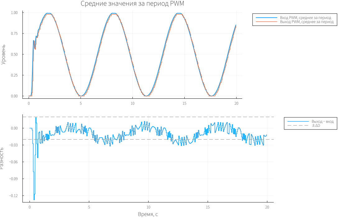
The upper graph shows the tracking of the average value for the input, the lower one shows the deviation.
We will output the measured errors, SQNR and delay.
println("Quantization step q:                    ", q)
println("max |quant_error| / q:                ", round(maximum(abs.(quant_error)) / q, digits = 3))
println("СКЗ quant_error / (q/√12):            ", round(rms(quant_error) / (q / sqrt(12)), digits = 3))
println("max |pcm_error| / q:                  ", round(maximum(abs.(pcm_error)) / q, digits = 3))
println("Percentage of samples with encoder saturation, %: ", round(100share, digits = 2))
println("Задержка фильтра: расчёт / данные, с: ", round(τ_filter, digits = 3), " / ", τ_est)
println("Average (output − input) PWM:           ", round(mean(pwm_dev), digits = 4))
@assert maximum(abs.(quant_error)) <= q/2 + 1e-8
@assert all(isfinite, d_k) && all(isfinite, pwm_dev)
string("PCM PWM passed; samples=", length(t_k), "; SQNR=", round(sqnr_quant; digits=1), " dB")
Conclusion
The model shows the effect of quantization and PCM range limitation on the accuracy of signal reconstruction. The quantization error does not exceed half a step, the filter delay is about 0.17 s, and the average PWM value follows the input signal.