Construction and analysis of logarithmic amplitude-phase frequency characteristics

Introduction

Logarithmic amplitude-phase frequency characteristics (LFCS) are one of the key tools for analyzing and synthesizing linear systems. They make it possible to visually assess the stability, speed and quality of regulation, as well as to investigate the influence of individual links on the behavior of the system as a whole. In modern engineering practice, automation of the construction of the LCF with the help of computing tools significantly speeds up the design and analysis process.

This example shows the implementation of an algorithm for constructing a frequency response using the ControlSystems library, which makes it possible to quickly investigate the frequency properties of various typical links and their combinations.

Importing libraries

We will attach the necessary libraries. To build the LFCH, we will need a library ControlSystems.

# EngeePkg.purge()
# import Pkg
# Pkg.add("ControlSystems")
using ControlSystems

The function for constructing the LFCH

The transfer function (fractional expression with coefficients) is formed using the function tf(); the vector of amplitudes, phase shifts, and cyclic frequencies is formed using the function bode() from the library ControlSystems. The construction of the LFCH is carried out on the basis of such data as:

Initial frequency
Final frequency
coefficients of the numerator polynomial
coefficients of the denominator polynomial.

Let's create a function for plotting the frequency response, in which we calculate the optimal frequency range for displaying on graphs and designate the scale type as logarithmic.

gr()
function LFCH(Numerator, Denominator, Low Frequency, High Frequency)
    A, F, ω = bode(tf(Numerator, Denominator), 2π.*range(Woofer, Hf, length = Int64(20*Hf/Woofer)))
    АЧХ = plot(ω./2π, 20 .* log10.(vec(A)), xscale = :log10, ylabel = "Amplitude, dB", title = "Frequency response")
    ФЧХ = plot(ω./2π, vec(Ф), xscale = :log10, title = "FCH", xlabel = "Frequency, Hz", ylabel = "Phase, °")
    AFC = plot(frequency response, FCH, layout=(2, 1), legend = false, lw = 2)
    display(AFC)
end

LFCH (generic function with 1 method)

Construction of the LFCH

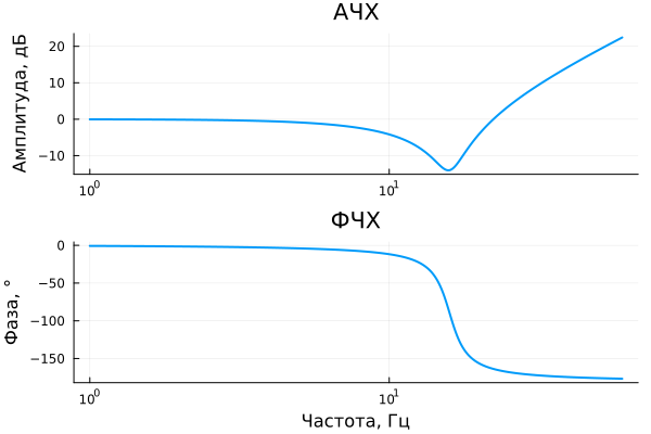
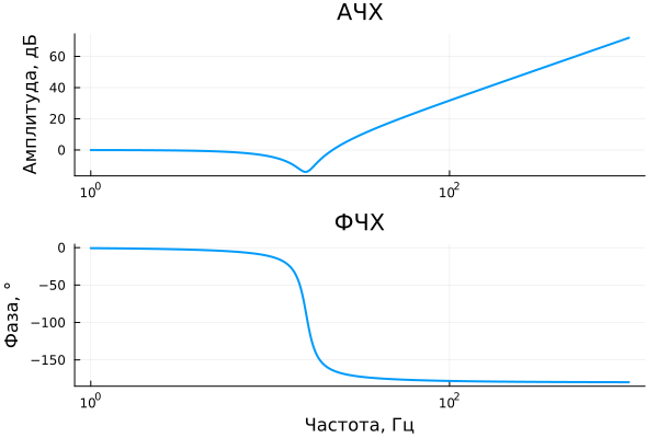
The transfer function is one of the ways to mathematically describe a system. The coefficients of the transfer function are listed in a numeric vector as multipliers of the polynomial of the largest power of the transfer function operator. to the smallest. The last (or only) coefficient will be the multiplier of the operator to the power of zero (one). Let's define the coefficients of the numerator and the coefficients of the denominator.

The numerator = [1, 5, 50, 500]
The denominator = [1000, 100, 10, 1]

With these coefficients, the transfer function will have the following form:

Let's determine the initial and final frequencies and build the frequency response.

Woofer = 1
Kh = 60
Low Frequency Response(Numerator, Denominator, Low Frequency, High Frequency)

Let's consider the LFCS of various typical elementary links.

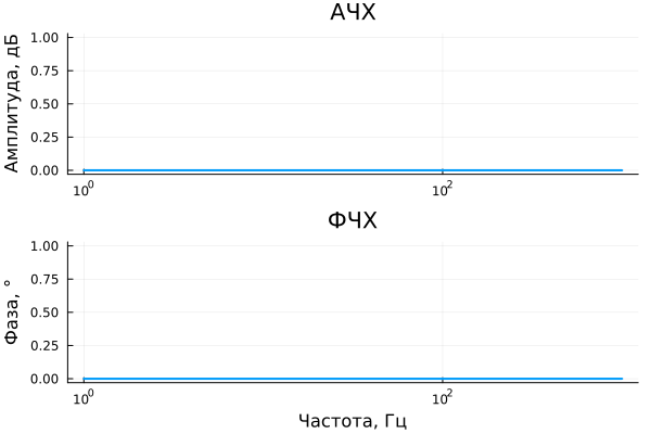
Proportional:

When the transfer function is equal to one:

we get the LCF of the proportional link.

# the propotional
Numerator = [1]
Denominator = [1]
Woofer = 1
Kh = 1000
Low Frequency Response(Numerator, Denominator, Low Frequency, High Frequency)

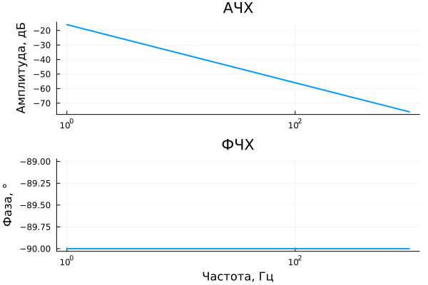
Perfectly integrating:

If the transfer function is inversely proportional to the operator :

we obtain the characteristic of an ideally integrating link.

# perfectly integrating
Numerator = [1]
Denominator = [1; 0]
Woofer = 1
Kh = 1000
Low Frequency Response(Numerator, Denominator, Low Frequency, High Frequency)

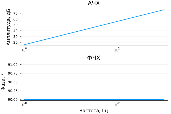
Perfectly differentiating:

When the transfer function is equal to the operator :

we obtain a characteristic of an ideally differentiating link.

# perfectly differentiating
Numerator = [1; 0]
Denominator = [1]
Woofer = 1
Kh = 1000
Low Frequency Response(Numerator, Denominator, Low Frequency, High Frequency)

Let's consider the links with the most complex shapes of the LCF.

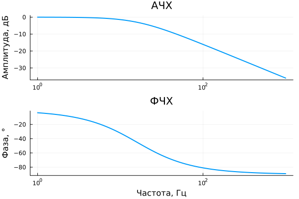
Aperiodic:

# aperiodic
Numerator = [1]
Denominator = [0.01; 1]
Woofer = 1
Kh = 1000
Low Frequency Response(Numerator, Denominator, Low Frequency, High Frequency)

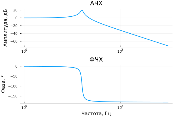
Periodic:

# periodic
Numerator = [1]
Denominator = [0.0001; 0.001; 1]
Woofer = 1
Kh = 1000
Low Frequency Response(Numerator, Denominator, Low Frequency, High Frequency)

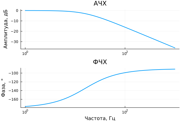
Unstable aperiodic:

# unstable aperiodic
Numerator = [1]
Denominator = [0.01; -1]
Woofer = 1
Kh = 1000
Low Frequency Response(Numerator, Denominator, Low Frequency, High Frequency)

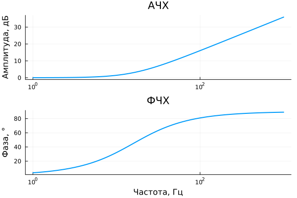
First-order differentiating:

# differentiating of the 1st order
Numerator = [0.01; 1]
Denominator = [1]
Woofer = 1
Kh = 1000
Low Frequency Response(Numerator, Denominator, Low Frequency, High Frequency)

Second-order forcing:

# forcing of the 2nd order
Numerator = [0.0001; -0.002; 1]
Denominator = [1]
Woofer = 1
Kh = 1000
Low Frequency Response(Numerator, Denominator, Low Frequency, High Frequency)

Conclusion

The presented example demonstrates an effective approach to the construction and analysis of linear systems using modern development tools. Using the ControlSystems library provides high computing speed, flexibility of configuration, and clarity of results. The LFCH construction function is the basis for creating interactive applications (digital stands) that will identify key features of systems and assess their dynamic stability over a wide frequency range. The considered examples cover the main types of elementary links, which makes it possible to apply the proposed approach to solve a wide range of problems in the theory of automatic control and related fields.