Determination of the frequency response using a pseudorandom binary sequence signal generator block
To build the frequency characteristics of the system, it is necessary to obtain the frequency response of the model: apply a test signal to the input of the system and measure its output. To reduce the time of the experiment, without losing the quality of the results, you can send a pseudorandom binary sequence (PRBS) signal instead of a harmonic signal. A PRBS is a periodic signal that can take only two specific values.
In this example, in the model_analysis_with_prbs.engee model, a PRBS signal is sent using special blocks and the system response is recorded. In this script, the data is processed and the LFCS is built.
Pkg.add("ControlSystems")
Pkg.add("DSP")
using ControlSystems
using DSP
using EngeeDSP
The sampling period of the algorithm
Ts = 0.001 # @param {type:"number"}
;
An array of frequencies at which the frequency response will be collected on a logarithmic scale.
wmin - the minimum frequency at which to build the LFCH
wmax is the maximum frequency at which to build the
LFCH n_ponts is the number of points on the graph.
wmin = 0.01 # @param {type:"number"}
wmax = 100 # @param {type:"number"}
n_points = 20 # @param {type:"number"}
w = collect(logrange(wmin, wmax, length=n_points));
Running the simulation
modelName = "model_analysis_with_prbs" # @param {type:"string"}
;
if modelName ∉ getfield.(engee.get_all_models(), :name)
    engee.load("$(@__DIR__)/$(modelName).engee");
end
engee.run(modelName);
Writing simulation data to variables
model_data = collect(PRBSSigGenData);
t = model_data[:,1];
data = model_data[:,2]

nd = size(data, 1)
nw = length(w)

ready = zeros(nd)
perturbation = zeros(nd)
input = zeros(nd)
output = zeros(nd)

for i = 1:nd
    ready[i] = data[i][1]
    perturbation[i] = data[i][2]
    input[i] = data[i][3]
    output[i] = data[i][4]
end
We process the signals before calculating the frequency response of the system
ts = t[2] - t[1]
dupidx = findall(diff(t) .< ts/2)
deleteat!(ready, dupidx)
deleteat!(perturbation, dupidx)
deleteat!(input, dupidx)

idx = findall(ready .== 1.)
d = perturbation[idx]
u = input[idx]
y = output[idx]

nfft = sum(idx .> 0.)

if !iszero(rem(nfft, 2))
    freq = (2*pi/ts) .* collect(range(0., 1., nfft + 1))
    lastel = Int64((nfft + 1) / 2)
    freq = freq[1:lastel]
else
    freq = (pi/ts) .* collect(range(0., 1., Int64(nfft/2) + 1))
end

pd = 2*pi / (nfft - 1)

filterwindow = [0.5 .* ones(nfft-1) .- 0.5 .* cos.(pd .* collect(0:nfft-2)); 0.]

fd = EngeeDSP.Functions.fft(d .* filterwindow);
fu = EngeeDSP.Functions.fft(u .* filterwindow);
fy = EngeeDSP.Functions.fft(y .* filterwindow);

d2u = fu ./ fd;
d2y = fy ./ fd;
u2y = d2y ./ d2u;
Constructing the frequency response
We get the frequency response of the system
Please note that the folder must contain a file with the function interpfreqresp.jl
# Connecting the file with the service function
include("$(@__DIR__)/interpfreqresp.jl")
plant_response = interpfreqresp(freq, u2y[1:length(freq)], w);
We calculate the frequency response of the system based on the frequency response
magnitude_estimated = 20 * log10.(abs.(plant_response));
phase_estimated = rad2deg.(DSP.unwrap((atan.(imag.(plant_response), real.(plant_response)))));
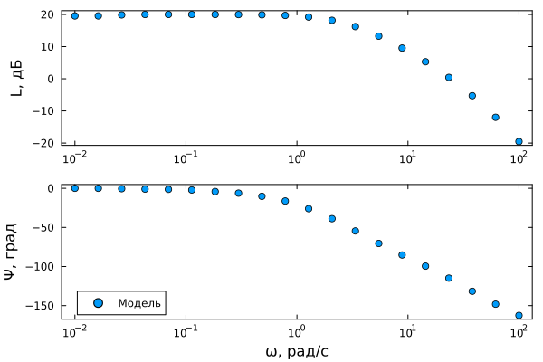
We are building a low-frequency response system
gr()
p1 = plot(w, magnitude_estimated, linealpha = 0.0, markershape = :circle, markersize = 4, ylabel = "L, dB", legend = :none)
p2 = plot(w, phase_estimated, linealpha = 0.0, markershape = :circle, markersize = 4, label = "Model", xlabel = "Oh, I'm glad/s", ylabel = ", hail", legend = :bottomleft)
plot(p1, p2, layout = (2,1), grid = false, framestyle = :box, xscale=:log10)
We calculate the frequency response of the transfer function of the system.
Let's compare the experimental LCF with the characteristic constructed by the transfer function.
# Management object
L = 0.006   # Inductance Gn
k = 0.10    # Counter-EMF coefficient (In⋅s)/rad
R = 0.25    # Ohm Resistance
J = 0.015   # Moment of inertia of the rotor kg⋅m^2
K = 0.10    # Torque constant N⋅m/A
tfnum = [K];
tfden = [L*J, R*J, K*k];
sys = tf(tfnum, tfden)
W = sys
W = c2d(sys, Ts) # We discretize the transfer function with a quantization period equal to the sampling period of the algorithm.
magnitude_ideal, phase_ideal, w_ideal = bode(W);
magnitude_ideal = reshape(magnitude_ideal, size(magnitude_ideal, 3),)
phase_ideal = reshape(phase_ideal, size(phase_ideal, 3),);
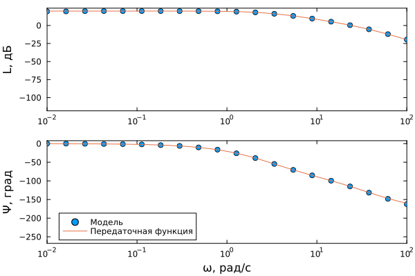
Comparison of LFCH
p1 = plot(w, magnitude_estimated, linealpha = 0.0, markershape = :circle, markersize = 4, ylabel = "L, dB", legend = :none)
plot!(w_ideal, 20 * log10.(magnitude_ideal), xlims = (wmin, wmax))
p2 = plot(w, phase_estimated, linealpha = 0.0, markershape = :circle, markersize = 4, label = "Model", xlabel = "Oh, I'm glad/s", ylabel = ", hail", legend = :bottomleft)
plot!(w_ideal, phase_ideal, xlims = (wmin, wmax), label = "Transfer function")
plot(p1, p2, layout = (2,1), grid = false, framestyle = :box, xscale=:log10)