Automated adjustment of the regulator
Introduction
Setting up a regulator for a control system is a classic task that is studied as part of a TAU course. However, all the methods that are studied in this course take a lot of time. In this publication, we will look at the application of optimization algorithms to speed up and automate control settings.
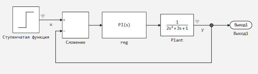
We will use the stepfun model for the demonstration.:
Preparatory work
We will need two libraries: ControlSystemBase and Optim. Let's install them:
import Pkg
Pkg.add(["ControlSystemsBase","Optim"])
Now, let's create a function to simulate the model. The simulation results will be passed to the stepinfo() function from ControlSystemBase. This function calculates the characteristics of the transition process and generates a StepInfo type object that can be visualized. We will return such an object:
gr()
engee.load(joinpath(@__DIR__,"stepfun.engee"))
using ControlSystemsBase
function sim_parameterized()
    simres = engee.run("stepfun")
    y = collect(simres["y"]);
    u = collect(simres["u"]);
    yv = reshape(y.value,(1,length(y.value)))
    rt = ControlSystemsBase.SimResult(yv,y.time,yv,u.value,ss(tf([1.0],[1.0, 0.0])))
    si = stepinfo(rt)
    return si
end
Getting started
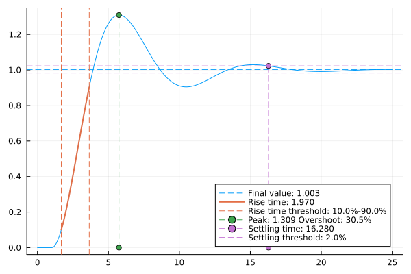
Let's look at how the system works with the default settings of the controller.:
    engee.set_param!("stepfun/reg","P"=>1.0)
    engee.set_param!("stepfun/reg","I"=>1.0)
    si = sim_parameterized()
    ref = plot(si)
    display(ref)
Let's explore the system by iterating through the parameters
Iterating through parameters is a fairly common method for investigating the effect of a parameter on the behavior of a system. The disadvantage of this method is that it takes a long time to iterate through the parameters. Even if we parallelize the search, we will wait an unacceptably long time for the result on large samples. And if the parameter varies in large leaps, the quality of the analysis will decrease. But even this can help in our task. Let's see what effect a change in the gain factor in the integrating link of the regulator will have.:
par_variation_l = 10;
param = collect(range(0.5,4.5,par_variation_l));
using ControlSystemsBase
# mySystem = feedback(tf([1.0],[1.0,1.0])*tf([1.0],[1.0, 0.0]))

K = 1.0

overshoot = zeros(par_variation_l);
setting_time = zeros(par_variation_l);
rise_time = zeros(par_variation_l);

for i in 1:par_variation_l
    engee.set_param!("stepfun/reg","I"=>"$(param[i])")
    si = sim_parameterized()
    overshoot[i] = si.overshoot;
    setting_time[i] = si.settlingtime;
    rise_time[i] = si.risetime;
end
Let's examine the results of iterating through the parameters
The easiest way to explore any data is to look at it through their eyes. Let's look at the overshoot (overshoot), rise time (rise_time), and setpoint time (setting_time) graphs.
p1 = plot(param, overshoot,label="overshoot")
p2 = plot(param,rise_time,color=:red,label="rise_time")
p3 = plot(param,setting_time,color=:green,label="setting_time")
plot(p1,p2,p3,layout=(3,1))
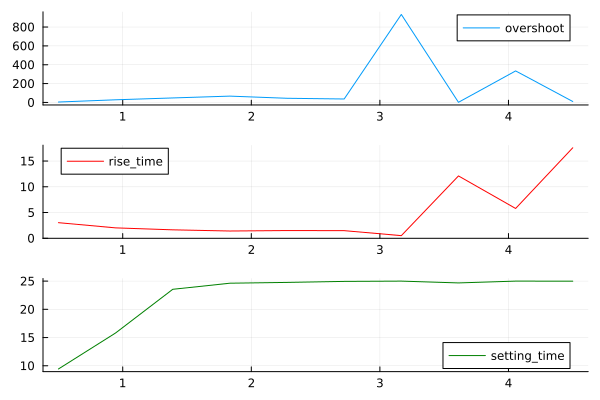
What matters here is not quantitative results, but how the system behaves. We see that as the gain in the integration link increases, overshoot and setpoint time increase. Thus, we can say that the desired optimal coefficient should be less than 1.5. If we carry out such an analysis for the starting link, then we will also be able to put forward a requirement for its reinforcement coefficient.
Automatic adjustment of the regulator parameters
We will use optimization methods to automatically adjust the regulator.
To apply optimization, you need to create an objective function, which we will look for the minimum. Let's use the StepInfo object to get the characteristics of the transient process from the results, and the function will return the sum of these characteristics multiplied by the weights. Weights are assigned based on the requirements for the transition process. Let's say we want to reduce the setpoint time while minimizing overshoot, but the rise time is not important to us. Then, our objective function will take the form:
function cost_fun(p::Vector{Float64})

    engee.set_param!("stepfun/reg","P"=>p[1])
    engee.set_param!("stepfun/reg","I"=>p[2])
    si = sim_parameterized()

    return 2*si.overshoot + 0.5*si.risetime + 10*si.settlingtime
end
Before you can start optimization and adjust the controller, you need to adjust the optimization itself. We want to limit the search for parameters, since we found out that the parameters have values less than 1.5. And their lower bound will be 0.5. Next, we need to limit the algorithm itself.
The optimization task will use two algorithms at once - Fminbox as the "external" one, and gradient descent as the "internal" one. At each step of the external algorithm, several steps of the internal algorithm will be run, and if we do not limit the number of steps of both algorithms, then optimization will take a long time or even freeze. For a more detailed description of the settings, refer to the documentation.
After completing all the settings, we will start optimization.:
using Optim
lowbound = [0.5, 0.5];
highbound = [1.5, 1.5];
opt = Optim.Options(
	iterations = 5,
	outer_iterations = 25,
	f_abstol = 1e-5,
	f_reltol = 1e-2,
	show_trace = true);
res = optimize(cost_fun, lowbound, highbound, [1.0, 1.0], Fminbox(GradientDescent()),opt)
The following values were found.
optimal_params = Optim.minimizer(res)
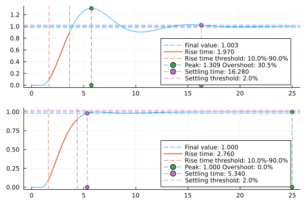
Let's build graphs of transients for the initial and configured regulators.:
    engee.set_param!("stepfun/reg","P"=>optimal_params[1])
    engee.set_param!("stepfun/reg","I"=>optimal_params[2])
    si = sim_parameterized()
    fin = plot(si)
    plot(ref,fin,layout=(2,1))
Conclusions
We looked at the process of automating the adjustment of the regulator. By iterating through the parameters, the boundaries within which the parameters of the regulator lie were obtained, and then their exact values were found.