Synthesis of the regulator
An example from the webinar "Engee capabilities for modeling Control Systems"
using ControlSystems
Ways to connect systems
W1 = tf(10, [9, 0.04, 0.01]);
W2 = tf(15, [2, 0.01, 0.7]);
Serial connection
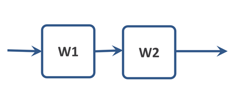
W = W1 * W2
W = series(W1, W2)
Parallel connection

W = W1 + W2
W = parallel(W1, W2)
Serial controller
In the first example, we will use the frequency characteristics to select a serial controller.
Management object
s = tf("s")
sys = (1s+2)/(0.2*s^2 +1.2*s+1)
Characteristics of the Management Object
p1 = ControlSystems.marginplot(sys)
p2 = plot(stepinfo(step(feedback(sys),0:0.01:5); settling_th=0.05), legend=:bottomright)
plot(p1, p2, layout = (1, 2))
Requirements:
- No static error
- Overshoot <15%
- Transition time <2 s
- Phase margin >60°
The regulator is an integrating link
A system with zero astaticity order, therefore, in order to meet the requirement of no static error, we will first add an integrating link as a regulator.:
controller = 1/s
p1 = ControlSystems.marginplot(sys*controller)
p2 = plot(stepinfo(step(feedback(sys*controller),0:0.01:10); settling_th=0.05), legend=:bottomright)
plot(p1, p2, layout = (1, 2))
The regulator is an integrating link + Gain factor
The system has become accurate. But it's quite slow, so we'll add a gain factor.
k = 5.6 # @param {type:"slider",min:0,max:10,step:0.1}
controller = k*1/s
p1 = ControlSystems.marginplot(sys*controller)
p2 = plot(stepinfo(step(feedback(sys*controller),0:0.01:5); settling_th=0.05), legend=:bottomright)
plot(p1, p2, layout = (1, 2))
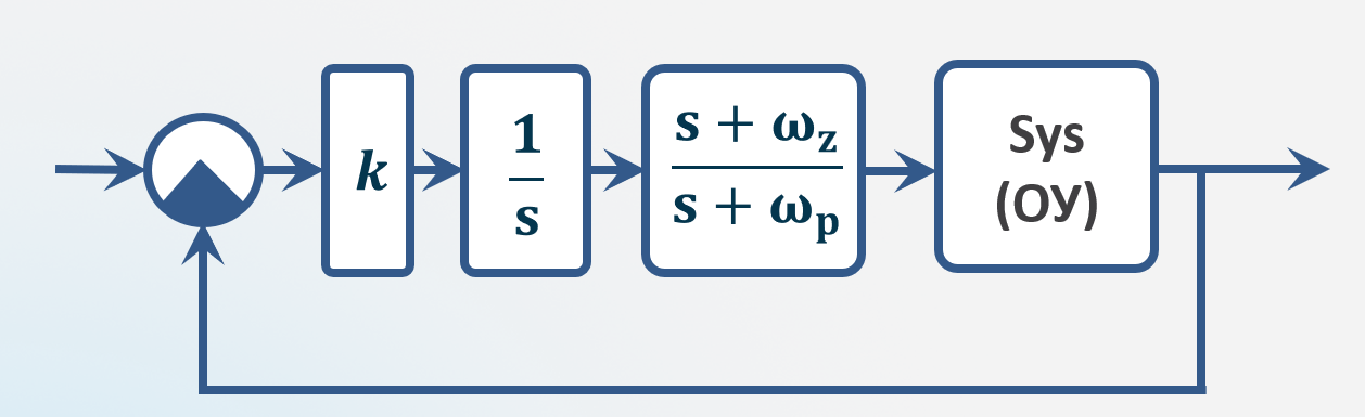
The regulator is an integrating link + Gain factor + Sequential phase-ahead correction device
It remains to increase the phase margin. It is necessary to change the slope of the frequency response in the medium frequency range in order to increase the stability of the system. To do this, we will add a sequential phase-ahead correction device.
wz = 6.6 # @param {type:"slider",min:1,max:10,step:0.1}
wp = 20.6 # @param {type:"slider",min:1,max:100,step:0.1}
k = 6.8 # @param {type:"slider",min:0,max:10,step:0.1}
controller = k*1/s*(s+wz)/(s+wp)
p1 = ControlSystems.marginplot(sys*controller)
ControlSystems.bodeplot!(sys*k*1/s)
p2 = plot(stepinfo(step(feedback(sys*controller),0:0.01:5); settling_th=0.05), legend=:bottomright)
annotate!(p2, 2, 0.8, text("Regulator = $k*s*(s + "* string(round(1/wz, digits=3))*")/(s + "*string(round(1/wp, digits=3))*")", :left, 8, :black))
plot(p1, p2, layout = (1, 2))
The resulting controller parameters can also be used in the model, for example, in the block Zeros and poles of the transfer function. You can verify this by examining the model. synthesis.engee.
The PID controller
using EngeeControlSystems
PID controller in parallel form
kp = 1.0
ki = 1.0
kd = 1.0
Tf = 0.01
pid_prl = Pid(kp, ki, kd, Tf) # continuous PID controller with first-order filter
PID controller in standard form
kp = 1.0
ti = 1.0
td = 1.0
n = 100
ts = 0.01
pid_std = PidStd(kp, ti, td, n, ts) # discrete PID controller with first-order filter
discr = c2d(pid_prl, ts)
d2c(discr)
Ts_new = 0.02
d2d(pid_std, Ts_new)
Auto-tuning the PID controller
pi_c, info = pidtune(sys, :pi, :parallel)
Wzam = feedback(pi_c*sys)
t = 0:0.005:12.0
plot(stepinfo(step(Wzam, t)))
Wraz = pi_c*sys
ControlSystems.marginplot(Wraz)
The result of the function pidtune it can be used in the model, for example, in the parameters of the PID controller block: Proportional coefficient: pi_c.kp and the Integral coefficient: pi_c.ki. An example is shown in the model synthesis.engee.