Variance analysis of mixed effects based on the example of data on the specific range of cars

Introduction

Imagine that you are a test engineer, and you need to find out whether different car models really differ in specific power reserve, or whether the observed differences are just an accident related, for example, to the specifics of a particular factory. The answer to this question is provided by analysis of variance, a statistical method that decomposes the overall variability of data into parts caused by different sources. The key idea is as follows: if the differences between the groups significantly exceed the level of random "noise", the influence of the factor is recognized as significant.

This example uses a mixed linear model. Each car model acts as a fixed effect, and the manufacturer and the interaction of the factory with the model act as random effects.

The result of training the model is the variance components, which quantify the contribution of each source to the overall spread.:

(Manufacturer) — how different are the cars from different factories on average;
(Manufacturer × Model) — the degree of inconsistency of the effect of the model from plant to plant (interaction of factors);
(Remainder) is an unexplained variation related to the individual characteristics of cars and measurement errors.

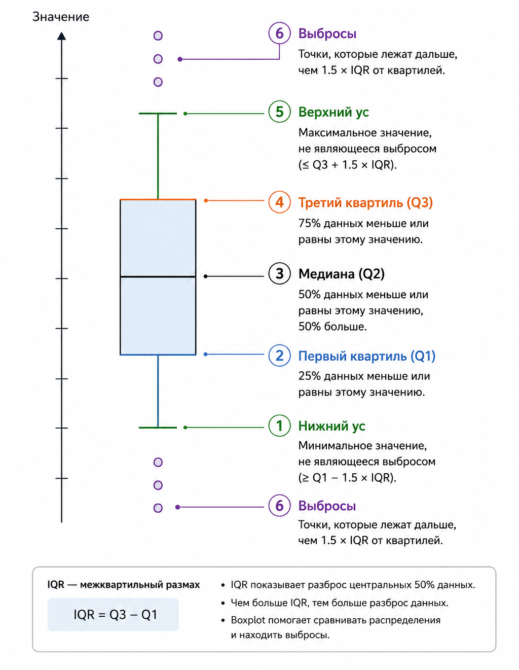
To visually represent the data, we use boxplots (boxplot, or "box with a mustache"). This graph compactly displays the median, quartiles, range, and potential outliers, allowing you to instantly estimate the center of the distribution, its spread, and symmetry in each group.

Formal hypothesis testing relies on the likelihood ratio test: it compares the complete model with a reduced (no fixed effect model) and determines whether the exclusion of the car model leads to a statistically significant deterioration in the description of the data.

By combining the capabilities of variance analysis of mixed effects with expressive statistical graphics, we reconstruct the objective picture hidden behind the columns of numbers in the test reports.

Importing libraries

We will add the libraries necessary for working with variance analysis.

# import Pkg
# Pkg.add(["AnovaGLM", "CSV", "DataFrames", "CategoricalArrays", "MixedModels", "Statistics", "Distributions", "GLM", "StatsPlots"])
using AnovaGLM, CSV, DataFrames, CategoricalArrays, MixedModels, Statistics, Distributions, GLM, StatsPlots

Initial data

Let's determine the initial data on the specific power reserve of each car model (пробег). We transform the data into a table in which the data is aligned.

# Initial data
source = [
    33.3  34.5  37.4
    33.4  34.8  36.8
    32.9  33.8  37.6
    32.6  33.4  36.6
    32.5  33.7  37.0
    33.0  33.9  36.7
]

# Experimental plan parameters
factories = 3
rows = 6
models = 2
repeats = div(rows, models)  
mileage = Float64[]
factory = Int[]
model = Int[]

force in 1:factories
    for page in 1:lines
        push!(mileage, initial[page, s])
        push!(factory, z)
        push!(model, page <= 3 ? 1 : 2)
    end
end

# Data table
table = DataFrame(
    Mileage = mileage,
    Factory = string.(factory),
    Model = string.(model)
)
table.Factory = categorical(table.Factory)
table.Model = categorical(table.The model)

println("Specific power reserve of cars")
println(first(table, 18))

Specific power reserve of cars
18×3 DataFrame
 [1m Row │ [1m Mileage [1m Factory [1m Model
     │ Float64  Cat…   Cat…
─────┼────────────────────────
   1 │    33.3  1      1
   2 │    33.4  1      1
   3 │    32.9  1      1
   4 │    32.6  1      2
   5 │    32.5  1      2
   6 │    33.0  1      2
   7 │    34.5  2      1
   8 │    34.8  2      1
   9 │    33.8  2      1
  10 │    33.4  2      2
  11 │    33.7  2      2
  12 │    33.9  2      2
  13 │    37.4  3      1
  14 │    36.8  3      1
  15 │    37.6  3      1
  16 │    36.6  3      2
  17 │    37.0  3      2
  18 │    36.7  3      2

Building models

Let's build a mixed linear model in which mileage is explained by the fixed effect of the car model and the random effects of the factory and the interaction of the factory with the model. Let's select the model parameters using the maximum likelihood method and analyze the obtained estimates of the variance components and fixed effects.

formula 1 = @formula(Mileage ~ 1 + Model + (1 | Factory) + (1 | Factory & The model))
fit1 = fit(MixedModel, formula 1, table)
println(selection 1)

Minimizing 2    Time: 0:00:00 ( 0.13  s/it)
   objective: 42.098336394833446

┌ Warning: ProgressMeter by default refresh meters with additional information in IJulia via `IJulia.clear_output`, which clears all outputs in the cell. 
│  - To prevent this behaviour, do `ProgressMeter.ijulia_behavior(:append)`. 
│  - To disable this warning message, do `ProgressMeter.ijulia_behavior(:clear)`.
└ @ ProgressMeter /usr/local/ijulia-core/packages/ProgressMeter/N660J/src/ProgressMeter.jl:607

Minimizing 34    Time: 0:00:00 (19.87 ms/it)

Linear mixed model fit by maximum likelihood
 Mileage ~ 1 + Model + (1| Factory) + (1 | Factory & The model)
   logLik   -2 logLik     AIC       AICc        BIC    
   -12.1071    24.2142    34.2142    39.2142    38.6661

Variance components:
                  Column   Variance Std.Dev. 
Factory & Model (Intercept) 0.000000 0.000000
Factory (Intercept) 2.948321 1.717068
Residual                    0.093778 0.306232
 Number of obs: 18; levels of grouping factors: 6, 3

  Fixed-effects parameters:
───────────────────────────────────────────────────
                 Coef.  Std. Error      z  Pr(>|z|)
───────────────────────────────────────────────────
(Intercept)  34.9444      0.996591  35.06    <1e-99
Model: 2 -0.566667 0.144359 -3.93 <1e-04
───────────────────────────────────────────────────

Let's build a reduced mixed model without a fixed effect of the car model, leaving only the random effects of the factory and interaction. Let's perform a likelihood ratio test between the full and reduced models in order to statistically verify the significance of the influence of the car model on mileage.

formula0 = @formula(Mileage ~ 1 + (1 | Factory) + (1 | Factory & The model))
fit0 = fit(MixedModel, formula0, table)
test_pravd = MixedModels.likelihoodratiotest(selection 0, selection 1)
println("Likelihood ratio test results:")
println(test_pravd)

Likelihood ratio test results:
Model Formulae
1: Mileage ~ 1 + (1|Factory) + (1 |Factory & The model)
2: Mileage ~ 1 + Model + (1|Factory) + (1|Factory & The model)
─────────────────────────────────────────────────
     model-dof  -2 logLik      χ²  χ²-dof  P(>χ²)
─────────────────────────────────────────────────
[1]          4    31.5367                        
[2]          5    24.2142  7.3224       1  0.0068
─────────────────────────────────────────────────

Estimates of variance components

Let's extract the variance components from the trained model using the function VarCorr Let's store the numerical variance values for each random effect in a convenient data structure.

components = VarCorr(selection 1)
println(components)
# A function for extracting variances
function extract the dispersion(vc)
    string_vc = string(vc)
    variances = Dict{String, Float64}()
    for line in split(строка_vc, "\n")
        cleaned = strip(line)
        if isempty(cleared)
            continue
        end
        if occursin("Variance components:", очищенная) || 
           occursin("Column", очищенная) || 
           (occursin("Variance", очищенная) && occursin("Std.Dev.", очищенная)) ||
           startswith(очищенная, "──")
            continue
        end
        
        части = split(очищенная, r"\s+")
        if length(parts) >= 3
            penultimate = parts[end-1]
            if occursin(r"^\d+\.?\d*$", предпоследнее) || occursin(r"^\d*\.?\d+$", предпоследнее)
                zn = tryparse(Float64, penultimate)
                if zn !== nothing
                    имя = join(части[1:end-2], " ")
                    variance[name] = zn
                end
            end
        end
    end
    return of variance
end

disp = extract the dispersions(components)
σ2_zavod = 0.0
σ2_interaction = 0.0
σ2_state = 0.0

for (k, v) int
    if occursin("Manufacturer & Model", k)
        σ2_interaction = v
    elseif occursin("Manufacturer", k) && !occursin("Model", k)
        σ2_zavod = v
    elseif occursin("Residual", k)
        σ2_state = v
    end
end

println("Estimates of random effect variances:")
println("  σ2(Manufacturer)                = ", round(σ²_завод, digits=4))
println("  σ2(Manufacturer:The model)         = ", round(σ²_взаимодействие, digits=4))
println("  σ2(Error)               = ", round(σ²_остаток, digits=4))

Variance components:
                  Column   Variance Std.Dev. 
Factory & Model (Intercept) 0.000000 0.000000
Factory (Intercept) 2.948321 1.717068
Residual                    0.093778 0.306232

Estimates of random effect variances:
  σ2(Manufacturer)                = 0.0
  σ2(Manufacturer:The model)         = 0.0
  σ2(Error)               = 0.0938

Visualization of results

Let's set up the visual design of the graphs.

theme(:default)
default(fontfamily="sans-serif", titlefontsize=11, guidefontsize=9, tickfontsize=7)
tsveta_zavodov = [:steelblue, :darkorange, :forestgreen]
color_comp = [:steelblue, :darkorange, :forestgreen]

3-element Vector{Symbol}:
 :steelblue
 :darkorange
 :forestgreen

Using boxplot, we will plot the distribution of the specific power reserve of cars for each manufacturer.

gr()
gr1 = @df boxplot table(:Factory, :Mileage,
    legend=false,
    title="Distribution of specific power reserve",
    xlabel="Manufacturer",
    ylabel="Specific power reserve",
    color=color_zavodov,
    linewidth=2,
    size=(500, 400))
display(gr1)

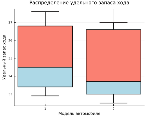
Let's plot the distribution of the specific power reserve of cars for each model.

gr2 = @df boxplot table(:Model, :Mileage,
    legend=false,
    title="Distribution of specific power reserve",
    xlabel="Car model",
    ylabel="Specific power reserve",
    color=[:salmon, :lightblue],
    linewidth=2,
    size=(500, 400))
display(gr2)

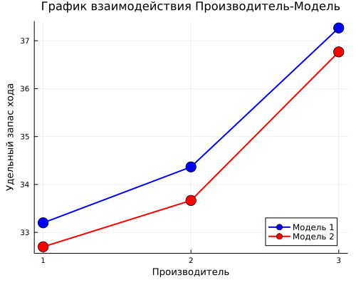
Let's build a graph of Manufacturer-Model interaction.

mean_zm = combine(groupby(table, [:Factory, :Model]), :Mileage => mean => :Average)
middle_ism.Factory = string.(average age.Factory)
middle_ism.Model = string.(average age.The model)
gr3 = plot(legend=:bottomright, size=(500, 400),
    title="Manufacturer-Model Interaction Schedule",
    xlabel="Manufacturer",
    ylabel="Specific power reserve")
colormodels = [:blue, :red]
for (i, мод) in enumerate(["1", "2"])
    data = average[average.Model.== mod, :]
    plot!(gr3, data.Factory, data.Average,
        marker=:circle, markersize=8, linewidth=2,
        color=color_models[i],
        label="The $mod model")
end
display(gr3)

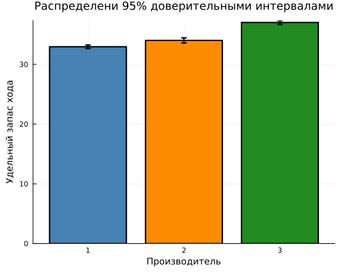
Let's group the data by manufacturer and calculate the specific power reserve, standard deviation, and number of observations for each one. Calculate the standard error of the mean and 95% confidence intervals. Let's build a bar chart with average values and error ranges in order to visually compare manufacturers by specific power reserve and evaluate the accuracy of the estimates obtained.

stat_zavod = combine(groupby(table, :Factory), 
    :Mileage => mean => :Average,
    :Mileage => std => :StOtkl,
    :Mileage => length => :N)
stat_zavod.Factory = string.(stat_zavod.Factory)
stat_zavod.Error = stat_zavod.Number/ sqrt.(stat_zavod.N)
stat_zavod.DI = 1.96 .* stat_zavod.A hundred mistakes

gr4 = bar(stat_zavod.Factory, stat_zavod.Average,
    yerror=stat_zavod.DEE,
    legend=false,
    title="Distributions with 95% confidence intervals",
    xlabel="Manufacturer",
    ylabel="Specific power reserve",
    color=color_zavodov,
    linewidth=2,
    size=(500, 400))
display(gr4)
println()

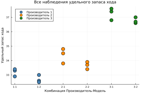
Let's construct a scattering diagram of all observations

таблица.Группа = string.(таблица.Завод) .* "-" .* string.(таблица.Модель)
table.Group = categorical(table.Group)
gr5 = plot(legend=:topleft, size=(600, 400),
    title="All observations of specific power reserve",
    xlabel="Manufacturer-Model Combination",
    ylabel="Specific power reserve")
for (i, з) in enumerate(["1", "2", "3"])
    data = table[table.Factory.== z, :]
    scatter!(gr5, data.Group, data.Mileage,
        label="Manufacturer $z",
        color=color_zavodov[i],
        markersize=8,
        markerstrokewidth=1.5)
end
display(gr5)

Let's build a heat map of the distribution of specific power reserve by models and manufacturers.

Matrix of averages = zeros(factories, models)
force in 1:factories
    for m in 1:models
        mask = (table.Factory.== string(h)) .& (table.Model.== string(m))
        matrix of averages[z, m] = mean(table.Mileage[mask])
    end
end
гр6 = heatmap(["Model 1", "Model 2"], 
    ["Manufacturer 1", "Manufacturer 2", "Manufacturer 3"],
    The matrix of averages, 
    title="Specific power reserve",
    xlabel="Model",
    ylabel="Manufacturer",
    color=:viridis,
    size=(400, 300))
display(gr6)

Conclusion

The analysis made it possible to quantify the variability of the specific power reserve into components related to the car model, the manufacturer and their interaction. The likelihood ratio test provided a formal answer to the question of the significance of the fixed effect of the model, and graphical support — from box diagrams to a heat map — made these conclusions clear and interpretable. Now a test engineer can rely not on intuition, but on statistically sound estimates: whether it is worth upgrading the design of the model or directing efforts to unify production processes between plants.

The considered method is universal and goes far beyond the automotive industry. In pharmaceuticals, it is used to assess the reproducibility of a drug's effect between different production sites: in agriculture, to separate the effect of plant variety, soil type and their interaction on yield; in psychology and education, when it is necessary to take into account both the individual differences of the subjects and the effect of experimental exposure. Wherever the data has a hierarchical structure (samples within batches, patients within clinics, students within classes), mixed models become an indispensable tool for correctly assessing the effects of interest and avoiding false conclusions due to ignoring the group structure of variability.

Thus, mastering the technique demonstrated in this example provides a universal opportunity for analyzing complexly organized data in a wide variety of subject areas.