Clustering of documents using the "bag of words" method
In this example, we will explore a way of presenting documents called a "bag of words" (BoW). This way of translating documents into numbers will allow us to translate each text into a vector representation. Despite the primitiveness of this vectorization method, it is possible to implement applied tasks based on it, provided that a suitable data set is available.
In this project, we will solve the clustering problem, which does not require training and test datasets, but simply divides the dataset into groups based on their coordinates in some space. First, we will study how to put texts into a homogeneous vector space, then how to saturate it with information, and finally how to see the result of clustering a set of texts.
# EngeePkg.purge()
Pkg.add(["XLSX", "Clustering", "MultivariateStats", "TextAnalysis", "SnowballStemmer", "StatsBase"])
using DataFrames, CSV, XLSX
using Statistics, StatsBase, LinearAlgebra, Clustering, Distances, MultivariateStats
using TextAnalysis, SnowballStemmer
stopwords_ru = CSV.read("$(@__DIR__)/stopwords.csv", DataFrame, header=0).Column1;
stemmer_ru = SnowballStemmer.Stemmer("russian");
We have prepared the environment and uploaded the necessary objects - a list of "stop words" that are skipped during the analysis and the simplest algorithm for detecting the root of a word (in order to get rid of word forms). Let's start downloading the texts.
Upload the texts
The data set that we will work with in this example will be a table with names and descriptions of examples from the Engee community. This is a set of small articles on various technical topics, from radio to economic calculations. The titles and short descriptions are written by the authors of the articles.
Let's see if we can use a primitive BoW to cluster these texts.
df = DataFrame(XLSX.readtable("$(@__DIR__)/Community.xlsx", "Community")) # Loading the table

titles = df.post_title
texts = df.post_title .* ". " .* df.post_description # We take the name and a short description

include("$(@__DIR__)/_scripts/doc_statistics.jl")
doc_statistics(texts)
We should immediately note that the texts are quite short. With a sufficiently variable dictionary, the information content of each text will be quite low.
Creating a case
The set of analyzed texts is called a corpus. They are both objects that fix the linguistic norm, and individual instances that can break out of it. First, we need to reduce the variability of words that occur. We will convert each text to lowercase (lowercase) and assemble the object. Corpus from objects StringDocument.
using TextAnalysis
corpus = Corpus( StringDocument.(lowercase.(texts)) )
update_lexicon!(corpus)
print("Words in the dictionary: $(length(corpus.lexicon))")
If we were to start working with this corpus now, each document could be represented by a vector of 5220 markers, each of which corresponds to the number of times a particular word occurs in the document. There are a lot more words than documents now. We need to simplify this space a bit. To do this, we will remove all numbers, spaces, and punctuation from the texts and reassemble the corpus.:
prepare!(corpus, strip_punctuation | strip_numbers | strip_whitespace )
update_lexicon!(corpus)
print("Words in the dictionary: $(length(corpus.lexicon))")
Let's remove stop words and words that are shorter than two characters from it.:
corpus.lexicon = Dict( (String(word), Int(freq)) for (word, freq) in corpus.lexicon if (length(word) > 2 && word ∉ stopwords_ru))
print("Words in the dictionary: $(length(corpus.lexicon))")
And the remaining words will be passed through a "stemmer" - an algorithm that cuts off typical word endings. Only cropped constructions will remain in the dictionary, which will sometimes match the root of the word. But we'll get rid of the word forms and be able to work with more unique constructions.
using StatsBase
corpus.lexicon = countmap([SnowballStemmer.stem(stemmer_ru, w) for (w,f) in corpus.lexicon for _ in 1:f])
print("Words in the dictionary: $(length(corpus.lexicon))")
Each document is characterized by a certain set of words. But for our analysis, we won't need unique words that don't occur in any other document. Let's discard them by filtering out those words from the dictionary that do not occur more than once in any document.
corpus.lexicon = Dict( (String(word), Int(freq)) for (word, freq) in corpus.lexicon if freq >= 2)
print("Words in the dictionary: $(length(corpus.lexicon))")
Function dtm() collects a matrix in which a set of words from the dictionary is assigned to each document.
dtm = DocumentTermMatrix(corpus) # Signs × Documents
We have 850 documents, many of which are characterized by the same words (vertical lines in the matrix), so in the final analysis we will see clusters around uninformative words like "work" or "example".
# BoW (frequency of words)
bow_dense = Matrix(dtm[:, :])'  # Признаки × Документы

# PCA
pca = fit(PCA, bow_dense; maxoutdim=3)
X_pca = MultivariateStats.predict(pca, bow_dense)  # (3, n_docs)

# Visualization (color = number of words in the document)
scatter(X_pca[1, :], X_pca[2, :], X_pca[3, :], legend=false,
        title="BoW projection", markersize=2, markerstrokewidth=0, alpha=0.7)
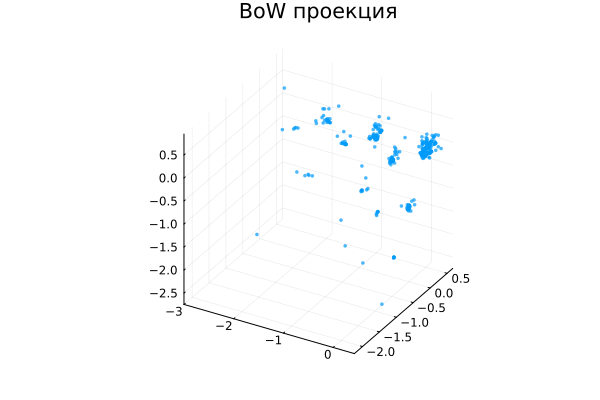
This is not a typical result for document clustering, although it would also be interesting to analyze it. Perhaps these are clusters along the length of the documents, and the variance arises from the fact that we projected the data into a reduced-dimensional space, losing some information about their variability, although the documents were very scattered in the original multidimensional space.
We have arranged all the documents in a 1,458-dimensional space. Naturally, to see them on the graph, we need to reduce the dimension, and the PCA analysis of the main components of the vector space will help us in this. It finds the projection in which the data is most variable.
To highlight the outstanding words, we will continue to work with a sparse representation of the text, but we will try to highlight the subject of each text. We will not establish connections between words (dense text analysis), but will raise the weight of some words relative to others.
Noise reduction using TFIDF
The next method that we need to try to apply is the method of "weighing" words in our bag, which is called TFIDF (term frequency, inverse document frequency). We will add weights to the words so that not all of them have the same meaning for analysis.
In our vector space, the documents will no longer be located in the same place as the rest of the documents where the word "work" is located. Along the axes of uninformative words, documents will slide closer to zero, and these axes will become uninformative.
The most expressive coordinates will be the numbers that characterize the presence of words in the document that are rarely found in the entire corpus. The more often a word occurs in a document and the less frequently it occurs in the corpus, the further away our document will be from zero in the coordinate corresponding to this dictionary word.
dtm = DocumentTermMatrix(corpus)
tfidf_mat = tf_idf(dtm)
A simple TFIDF document matrix looks the same as the frequency matrix after BoW, but we only see the presence or absence of a number, not its value. The most unique or specific words will gain more weight.
# Maximum weight per document (unique/specific words)
vocab = collect(keys(corpus.lexicon))
max_tfidf = maximum(tfidf_mat, dims=2)[:]
top_idx = sortperm(max_tfidf, rev=true)[1:10]
top_words = join(vocab[top_idx], ", ")
The problem is that we work with short texts. If there are from 2 to 23 words in a text (the average length is 13), then almost any words are rare and will look like noise. Nevertheless, let's see how our texts are arranged in space now.
tfidf_dense = Matrix(tfidf_mat)'; # Dimensions: Features × Documents

mean_vec = mean(tfidf_dense, dims=2)      # Center the data first
centered_data = tfidf_dense .- mean_vec

pca = fit(PCA, centered_data; maxoutdim=3)
X_pca = MultivariateStats.predict(pca, (tfidf_dense))  # (n_docs, n_components)

scatter(X_pca[1, :], X_pca[2, :], X_pca[3, :], title="Projection of the token space", leg=false,
                markersize=2, markerstrokewidth=0, alpha=0.7)

plot!(size=(1000,400), titlefont=font(8))
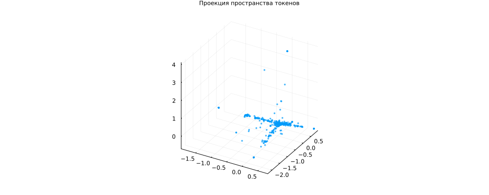
Interestingly, many tests are located in the middle of the coordinate system (not representative), but there are several "rays" - groups of words that occur together and characterize their groups of documents. This is a typical picture for the thematic modeling task.
Nothing guarantees that these groups of words are related to each other, we have a fairly small data set and short texts, the grouping may be the result of a random distribution.
In addition, this is a grouping after projection, there might not have been any "rays" in the original space. But the texts were definitely located at different distances from the origin.
Let's perform clusterization for the number of clusters we set.
# Clusterization
k = 5
clusters = kmeans(X_pca, k; distance=CosineDist(), maxiter=500)

# For each cluster, we find the top 3 most remote documents.
top_ids_list = Dict{Int, Vector{Int}}()
for cluster_id in 1:k
    idx_in_cluster = findall(clusters.assignments .== cluster_id)
    if isempty(idx_in_cluster); continue; end

    center = clusters.centers[:, cluster_id]
    distances = [norm(X_pca[:, i] - center) for i in idx_in_cluster]
    top_idx = idx_in_cluster[sortperm(distances, rev=true)[1:min(3, end)]]
    top_ids_list[cluster_id] = top_idx
end

# We draw each cluster with its legend separately
p = plot()
for cluster_id in 1:k
    idx_in_cluster = findall(clusters.assignments .== cluster_id)
    if isempty(idx_in_cluster); continue; end

    # Cluster name in the legend
    label = string("Class ", cluster_id, " (", join(top_ids_list[cluster_id], ", "), ")")

    scatter!(p, X_pca[1, idx_in_cluster], X_pca[2, idx_in_cluster], X_pca[3, idx_in_cluster],
             label=label, markersize=3, alpha=0.6)
end

plot!(p, title="Ray clustering (k=$k)", legend=:outertopright, size=(1000,600))
display(p)
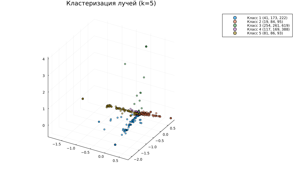
Cosine metric clustering, for centered data, allows us to cluster documents by their "spatial angle". We tried to make the individual rays fall into separate clusters.
Here are some of the most representative documents for each cluster.:
max_docs = 6

for cluster_id in 1:k
    idx_in_cluster = findall(clusters.assignments .== cluster_id)
    if isempty(idx_in_cluster); continue; end

    # Keywords for the cluster (peripheral documents)
    center = clusters.centers[:, cluster_id]
    distances = [norm(X_pca[:, i] - center) for i in idx_in_cluster]
    threshold = quantile(distances, 0.7)
    peripheral_idx = idx_in_cluster[distances .>= threshold]

    # Top 5 words from the periphery
    if !isempty(peripheral_idx)
        avg_tfidf = mean(tfidf_mat[peripheral_idx, :], dims=1)[:]
        top_idx = sortperm(avg_tfidf, rev=true)[1:min(5, end)]
        top_words = vocab[top_idx]
        keywords = join(top_words, ", ")
    else
        keywords = "—"
    end

    # Top 3 most deleted documents
    top_docs = idx_in_cluster[sortperm(distances, rev=true)[1:min(max_docs, end)]]

    println("\Cluster $cluster_id ($(length(idx_in_cluster)) dock, keywords: $keywords)")
    for (rank, idx) in enumerate(top_docs)
        println("  $rank. [$idx] $(titles[idx])")
    end
end
It's not that the differences are obvious. Let's look at the statistics:
# Let's check the sparsity of the matrix
println("Sparsity of TF-IDF matrix: $(1 - SparseArrays.nnz(tfidf_mat)/prod(size(tfidf_mat)))%")
println("Average number of non-zero elements per document: $(SparseArrays.nnz(tfidf_mat)/size(tfidf_mat, 1))")

# Let's look at the variance
row_variances = [var(collect(row)) for row in eachrow(tfidf_mat)]
println("Variance by documents: average $(mean(row_variances))")
println("                         median $(median(row_variances))")
println("                        min/max $(minimum(row_variances)) / $(maximum(row_variances))")
Our documents don't lend themselves very well to this kind of clustering. The high sparsity of the matrix means that very few documents can be grouped according to such a vector feature.
We also see that each document is characterized by an average of 1.8 unique words (our matrix has so many non-zero elements on average). This is very small, it is better to increase this figure to 5-10% of the vocabulary, but since our texts are very short, we will not be able to do this.
Having 1-2 significant words per document (after stemming), we get almost zero variance - all documents are very poor in information.
Conclusion
Sparse text analysis methods usually show good results in auxiliary tasks: spam filtering, identification of unique texts or symbols, comparison of documents with specific terminology, and basic clustering.
We have also studied the methods of text preprocessing that are used at every step, in every text analysis application project. As you can see, we can use a dozen functions to organize a relatively complex text processing chain.