Neural network forecasting of time series

Introduction

Time series forecasting is one of the fundamental tasks of data analysis that arises in economics, meteorology, energy, and many other fields. Classical statistical methods work well on linear dependencies, but they often fail to cope with complex nonlinear patterns. Neural networks offer a flexible alternative: They are able to automatically identify hidden patterns without explicitly specifying a model.

This paper demonstrates the simplest neural network approach to forecasting, trained in an autoregressive formulation. The model uses the two previous values of the series to predict the next one, and then iteratively builds a forecast for a given horizon. This approach serves as a visual starting point for exploring more complex neural network architectures.

Libraries used

We will attach the necessary libraries. To work with the neural network, we will need the Flux library.

using Flux, Random, LinearAlgebra, Statistics

Initial data

Let's define the initial data. Let's create a time series of 100 points: sinusoid + linear trend + noise. Normalize the series (subtract the average, divide by the standard deviation). Let's form a matrix of features.

Random.seed!(42)
# Data generation
t = 1:100
L = length(t)
z = 10*sin.(0.2*t) + 0.2*t + 0.3*randn(L)

# Normalization of data
z_mean = mean(z)
z_std = std(z)
z_norm = (z .- z_mean) ./ z_std  # normalized data

# Formation of the input matrix
x = zeros(2, L)
x[1, 2:end] = z_norm[1:end-1]  # z(t-1)
x[2, 3:end] = z_norm[1:end-2]  # z(t-2)
x_data = Float32.(x)
z_data = Float32.(z_norm)

Configuring a neural network

Let's create a neural network: input layer (2→8), hidden layer (8→4), output layer (4→1). Let's set up the Adam optimizer with a learning rate of 0.001 and link it to the network. We will prepare an array for recording errors at each epoch. Let's set 5000 training epochs.

net = Chain(Dense(2 => 8, relu), Dense(8 => 4, relu),Dense(4 => 1))
optimizer = Adam(0.001)
opt_state = Flux.setup(optimizer, net)
losses = Float32[]
epochs = 5000

Loss function

Let's create a loss function: we'll pass a matrix of features to the model input, get predictions, convert them into a one-dimensional vector, and calculate the root-mean-square error between the predictions and the true values.

function loss(model, x, y)
    y_pred = vec(model(x))
    return Flux.mse(y_pred, y)
end

Neural network training

Let's start the learning cycle: calculate the gradients and update the parameters. After training, we will get network predictions for all 100 points.

for epoch in 1:epochs
    current_loss = loss(net, x_data, z_data)
    push!(losses, current_loss)
    Flux.train!(net, [(x_data, z_data)], opt_state) do m, xb, yb
        loss(m, xb, yb)
    end
    if epoch % 100 == 0
        # println("Epoch $epoch: loss = $(round(current_loss, digits=6))")
    end
end

y_train_norm = vec(net(x_data))
y_train = y_train_norm .* z_std .+ z_mean

Time series forecast

We will get the predicted values of the time series for 50 points ahead.

function forecast(net, z_norm, z_mean, z_std, horizon=50)
    y_full_norm = zeros(Float32, 100 + horizon)
    y_full_norm[1:100] = z_norm
    for i in 1:horizon
        idx = 100 + i
        input_vec = Float32.([y_full_norm[idx-1], y_full_norm[idx-2]])
        y_full_norm[idx] = net(reshape(input_vec, 2, 1))[1]
    end
    return y_full_norm .* z_std .+ z_mean
end

y_full = forecast(net, Float32.(z_norm), z_mean, z_std, 50)

150-element Vector{Float64}:
  2.077686166487098
  4.369704383951254
  6.151928340143768
  7.8801850772692745
  9.659601907697848
 10.663412370556056
 10.99663069738901
 11.154949594543305
 10.904175864829527
 11.106108789428392
 10.037363671824608
  9.406718355367095
  7.885179545387794
  ⋮
  8.16153229190152
  9.871865117523257
 11.16291496603565
 11.63761469392388
 11.440856430263558
 10.529202720345774
  8.602405889069477
  6.954229163008996
  5.774611191033784
  4.69222943408103
  3.7329430285822243
  2.9190516942247546

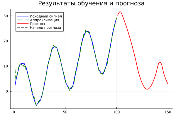
Visualization

Let's display the original signal, the approximation, and the forecast on the graph.

# Visualization
gr()
graph = plot(1:100, z, 
          label="The original signal", 
          color=:blue, 
          linewidth=2,
          title="Learning and forecasting results",
          legend=:topleft
          )
plot!(graph, 1:100, y_train, 
      label="The approximation", 
      color=:green, 
      linestyle=:dash,
      linewidth=2)
plot!(graph, 101:150, y_full[101:150], 
      label="Forecast", 
      color=:red,
      linewidth=2)
vline!(график, [100.5], label="The beginning of the forecast", color=:black, linestyle=:dash)

display(graph)

Conclusion

In this example, a fully connected neural network is implemented and trained to predict a model time series. Despite the simplicity of the architecture, the model successfully accepted both periodic and trend components of the signal, and also demonstrated the possibility of multi-valued forecasting in autoregressive mode.

In practice, neural network time series forecasting is used for:

predictions of commodity prices, stocks and exchange rates in trading systems;
forecasting electricity consumption for load balancing of power grids;
Estimating the demand for goods in trade for inventory management;
Meteorological modeling and short-term weather forecast;
monitoring the condition of industrial equipment based on telemetry data.

The presented script can serve as a basis for moving to more advanced architectures — recurrent and transformer networks, specially designed to work with sequential data.