Performance comparison of Julia and Matlab ensemble methods
Introduction
Modern machine learning tasks require not only high model accuracy, but also efficient use of computing resources. The choice of tools directly affects the speed of development and training time, which is especially critical when working with large amounts of data and ensemble methods known for their resource intensity.
Ensemble methods are machine learning methods that combine several basic models (for example, decision trees) to produce a more accurate and stable forecast than each model individually.
This example provides a comparative analysis of three approaches to learning a classification model based on a random forest.:
- using the MLJ and DecisionTree libraries on Julia,
- as well as the fitcensemble functions in the plug-in Matlab core.
All methods solve the same problem of binary classification on synthetic data, which allows an objective comparison of their performance.
Importing libraries
We will attach the necessary libraries.
import Pkg
Pkg.add(["Random", "Distributions", "LinearAlgebra", "Statistics", "DecisionTree", "MLJ", "MLJDecisionTreeInterface"])
using Random, Distributions, LinearAlgebra, Statistics
Data generation
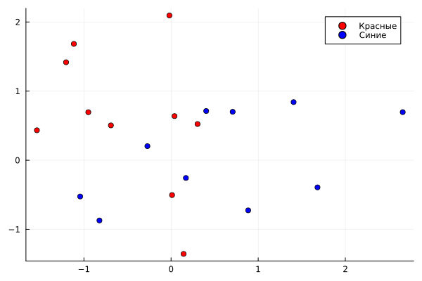
Let's create ten red and ten blue basepoints. Please note that in Julia you can use emoji characters in variable names.
🔴 = rand(MvNormal([0.0, 1.0], 1.0I), 10)'
🔵 = rand(MvNormal([1.0, 0.0], 1.0I), 10)'
Let's display the base points on the coordinate plane.
gr()
график1 = scatter(🔴[:, 1], 🔴[:, 2], color=:red, marker=:circle, label="Red", legend=:topright)
scatter!(🔵[:, 1], 🔵[:, 2], color=:blue, marker=:circle, label="Blue")
display(graph1)
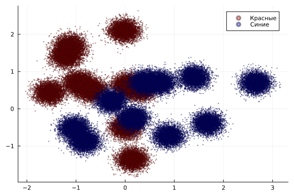
Create 50,000 dots of each color centered at random base points.
N = 50000

🔴 = 🔴[rand(1:10, N), :] + randn(N, 2) .* sqrt(0.02)
🔵 = 🔵[rand(1:10, N), :] + randn(N, 2) .* sqrt(0.02)

график2  =scatter(🔴[:, 1], 🔴[:, 2], color=:red, marker=:circle, markersize=1, label="Red", alpha=0.36, legend=:topright)
scatter!(🔵[:, 1], 🔵[:, 2], color=:blue, marker=:circle, markersize=1, label="Blue", alpha=0.36)
display(graph2)
Combine the data and create class labels for the classification task. Create a single vector of labels and assign a -1 label for the blue dots.
data = [🔴; 🔵]
tags = ones(2*N)
labels[N+1:2*N] .= -1
# red 1, blue -1
display(data)
Comparison of classification models
MLJ
Let's train the model using the tools of the MLJ library (Machine Learning in Julia).
using MLJ, MLJDecisionTreeInterface
tree = @load DecisionTreeClassifier pkg=DecisionTree
time = @elapsed begin
   model = MLJ.fit!(machine(EnsembleModel(model = tree(max_depth=-1), n=100, bagging_fraction=1.0, rng=1234),
    DataFrame(data, :auto), coerce(ifelse.(labels .== 1.0, 1, 2), Multiclass)))
end

display(model)
println("Training time: ", время, " seconds")
The training time of the model using MLJ was: 33.51 seconds.
Matlab fitensemble
Let's train the model inside the Matlab core using the function fitcensemble, and measure the execution time.
using MATLAB

cdata = data
grp = tags
@mput cdata grp N

mat"""
tic
mdl = fitcensemble(cdata, grp, 'Method', 'Bag');
stime = toc;
disp(mdl)
"""
@mget(stime)
println("Training time: ", stime, " seconds")
The training time of the model using Matlab was: 29.57 seconds.
DecisionTree
Let's train the model using the DecisionTree library tools.
using DecisionTree
time = @elapsed begin
model = build_forest(labels, data, 2, 100, 1.0, rng=Random.GLOBAL_RNG)
end
display(model)
println("Training time: ", время, " seconds")
The training time of the model using DecisionTree was: 6.07 seconds. This is the best result studied.
Conclusion
In this study, an ensemble of 100 decision trees was trained on synthetic data. A comparison of the three approaches showed a significant difference in performance.
The Julia DecisionTree native library (6.07 c) demonstrated the best performance, which makes it an excellent choice for high-load tasks and prototyping.
The results confirm that Engee provides significant performance gains compared to Matlab, while maintaining compatibility with its syntax. The presented classification methods are applicable in the tasks of computer vision, predictive analytics, medical diagnostics and financial modeling, where high accuracy and speed of processing large amounts of information are required.