Engee documentation
Notebook

Code generation from a model with nested subsystems.

This example logically continues the previous demonstration. Its purpose is to show the capabilities of the Verilog code generator, namely various approaches to structuring the final project through the use of atomic subsystems.

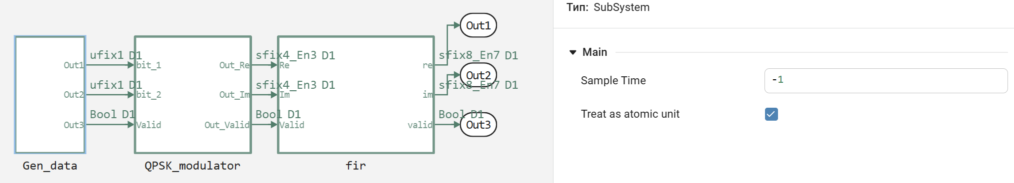
The figure below shows the implemented model. It contains the configuration "Treat as atomic unit" applied to only one of the two blocks, which allows you to visually compare the generation results.

image.png

Now let's move on to code generation and comparing the results with the original model. First, let's declare an auxiliary function that will run our model.

In [ ]:
function run_model( name_model)
    Path = (@__DIR__) * "/" * name_model * ".engee"
    if name_model in [m.name for m in engee.get_all_models()] # Проверка условия загрузки модели в ядро
        model = engee.open( name_model ) # Открыть модель
        model_output = engee.run( model, verbose=true ); # Запустить модель
    else
        model = engee.load( Path, force=true ) # Загрузить модель
        model_output = engee.run( model, verbose=true ); # Запустить модель
        engee.close( name_model, force=true ); # Закрыть модель
    end
    sleep(0.1)
    return model_output
end
Out[0]:
run_model (generic function with 1 method)

Now let's configure the model for code generation on Verilog.

image.png

We will perform code generation directly from the model interface (at the click of a button), so as not to overload the already voluminous script.

image.png

Next, we declare an auxiliary function for reading the generated Verilog files. How the function works read_v it consists of the following. First, it checks the existence of the specified file in the file system. If the file is not found, a corresponding message is displayed. Upon successful detection, the function reads the entire contents of the file as a string and visually outputs it to the console, framing it with a header and delimiters for ease of perception.

In [ ]:
function read_v(filename)
    try
        if !isfile(filename)
            println("Файл $filename не найден!")
            return
        end
        println("Содержимое файла $filename:")
        println("="^50)
        content = read(filename, String)
        println(content)
        println("="^50)
        println("Конец файла")
    catch e
        println("Ошибка при чтении файла: ", e)
    end
end
Out[0]:
read_v (generic function with 1 method)

Now let's move on to comparing the implementation of subsystems. The key difference is in the organization of the output code.

Без имени.png

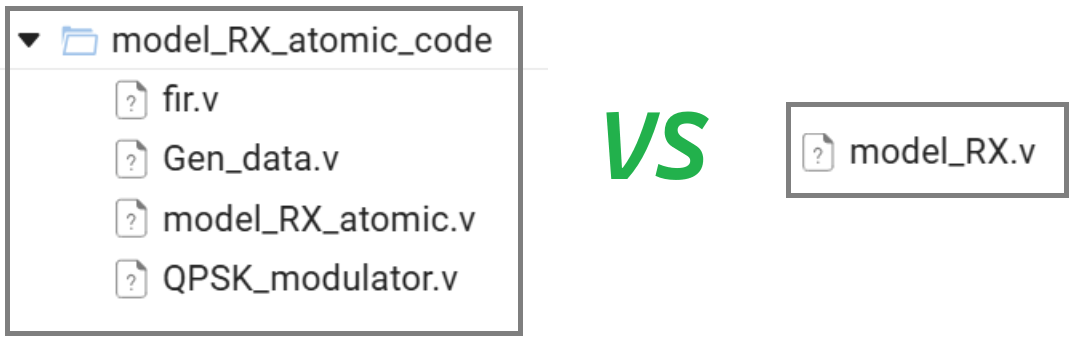
In the case of implementation without the use of atomic subsystems, the head project file includes all the logic of the system, presented as a single monolithic module. This module contains numerous registers and complex combination chains combined in a single namespace.

In [ ]:
read_v("$(@__DIR__)/model_RX.v")
Содержимое файла /user/start/examples/codegen/qpsk_and_fir_verilog_v2/model_RX.v:
==================================================
/* Code generated by Engee
 * Model name: model.engee
 * Code generator: release-1.1.22
 * Date: Wed Sep 10 06:27:06 2025 GMT
 */

module model_RX(
  input        clock,
               reset,
  output       io_Out3,
  output [7:0] io_Out1,
               io_Out2
);

  reg         UnitDelay_1_state;
  reg         UnitDelay_13_state;
  reg         UnitDelay_state;
  reg         UnitDelay_1_1_state;
  reg         UnitDelay_2_state;
  reg         UnitDelay_3_state;
  reg         UnitDelay_4_state;
  reg         UnitDelay_13_1_state;
  reg         UnitDelay_14_state;
  reg         UnitDelay_5_state;
  reg         UnitDelay_6_state;
  reg         UnitDelay_14_1_state;
  reg         UnitDelay_7_state;
  reg         UnitDelay_8_state;
  reg         UnitDelay_9_state;
  reg         UnitDelay_10_state;
  reg         UnitDelay_11_state;
  reg  [3:0]  UnitDelay_12_state;
  reg  [3:0]  UnitDelay_13_2_state;
  reg  [3:0]  UnitDelay_14_2_state;
  reg  [3:0]  UnitDelay_15_state;
  reg  [3:0]  UnitDelay_16_state;
  reg  [3:0]  UnitDelay_17_state;
  reg  [3:0]  UnitDelay_18_state;
  reg  [3:0]  UnitDelay_19_state;
  reg  [3:0]  UnitDelay_20_state;
  reg  [3:0]  UnitDelay_21_state;
  reg  [3:0]  UnitDelay_22_state;
  reg  [3:0]  UnitDelay_23_state;
  reg  [3:0]  UnitDelay_24_state;
  reg  [3:0]  UnitDelay_25_state;
  reg  [3:0]  UnitDelay_26_state;
  reg  [3:0]  UnitDelay_27_state;
  reg  [3:0]  UnitDelay_28_state;
  reg  [3:0]  UnitDelay_29_state;
  reg  [3:0]  UnitDelay_30_state;
  reg  [3:0]  UnitDelay_31_state;
  wire        LogicalOperator = UnitDelay_13_state ^ UnitDelay_14_state;
  wire        LogicalOperator_1 = UnitDelay_1_state ^ UnitDelay_14_1_state;
  wire [2:0]  _IdxAccum_T_2 =
    {1'h0, LogicalOperator, 1'h0} + {2'h0, LogicalOperator_1} + 3'h1;
  wire        _tmp6_T = _IdxAccum_T_2 == 3'h2;
  wire        _constellation_selector_im_T = _IdxAccum_T_2 == 3'h1;
  wire [3:0]  _constellation_selector_re_new_T_1 =
    _constellation_selector_im_T | ~(_tmp6_T | _IdxAccum_T_2 == 3'h3) ? 4'h6 : 4'hA;
  wire [3:0]  _constellation_selector_im_new_T_1 =
    _constellation_selector_im_T | _tmp6_T ? 4'h6 : 4'hA;
  wire [10:0] _Gain_1_new_T_1 =
    {{7{_constellation_selector_re_new_T_1[3]}}, _constellation_selector_re_new_T_1}
    * 11'h7FF;
  wire [10:0] _Gain_1_1_new_T_1 =
    {{7{_constellation_selector_im_new_T_1[3]}}, _constellation_selector_im_new_T_1}
    * 11'h7FF;
  wire [10:0] _Gain_3_new_T_1 =
    {{7{UnitDelay_14_2_state[3]}}, UnitDelay_14_2_state} * 11'h7FE;
  wire [10:0] _Gain_3_1_new_T_1 =
    {{7{UnitDelay_15_state[3]}}, UnitDelay_15_state} * 11'h7FE;
  wire [10:0] _Gain_5_new_T_1 =
    {{7{UnitDelay_19_state[3]}}, UnitDelay_19_state} * 11'h7FE;
  wire [10:0] _Gain_5_1_new_T_1 =
    {{7{UnitDelay_18_state[3]}}, UnitDelay_18_state} * 11'h7FE;
  wire [10:0] _Gain_6_new_T_1 = {{7{UnitDelay_21_state[3]}}, UnitDelay_21_state} * 11'h30;
  wire [10:0] _Gain_6_1_new_T_1 =
    {{7{UnitDelay_20_state[3]}}, UnitDelay_20_state} * 11'h30;
  wire [10:0] _Gain_7_new_T_1 =
    {{7{UnitDelay_22_state[3]}}, UnitDelay_22_state} * 11'h7FE;
  wire [10:0] _Gain_7_1_new_T_1 =
    {{7{UnitDelay_23_state[3]}}, UnitDelay_23_state} * 11'h7FE;
  wire [10:0] _Gain_9_new_T_1 =
    {{7{UnitDelay_27_state[3]}}, UnitDelay_27_state} * 11'h7FE;
  wire [10:0] _Gain_9_1_new_T_1 =
    {{7{UnitDelay_26_state[3]}}, UnitDelay_26_state} * 11'h7FE;
  wire [10:0] _Gain_11_new_T_1 =
    {{7{UnitDelay_30_state[3]}}, UnitDelay_30_state} * 11'h7FF;
  wire [10:0] _Gain_11_1_new_T_1 =
    {{7{UnitDelay_31_state[3]}}, UnitDelay_31_state} * 11'h7FF;
  always @(posedge clock) begin
    if (reset) begin
      UnitDelay_1_state <= 1'h0;
      UnitDelay_13_state <= 1'h0;
      UnitDelay_state <= 1'h0;
      UnitDelay_1_1_state <= 1'h0;
      UnitDelay_2_state <= 1'h0;
      UnitDelay_3_state <= 1'h0;
      UnitDelay_4_state <= 1'h0;
      UnitDelay_13_1_state <= 1'h1;
      UnitDelay_14_state <= 1'h0;
      UnitDelay_5_state <= 1'h0;
      UnitDelay_6_state <= 1'h0;
      UnitDelay_14_1_state <= 1'h1;
      UnitDelay_7_state <= 1'h0;
      UnitDelay_8_state <= 1'h0;
      UnitDelay_9_state <= 1'h0;
      UnitDelay_10_state <= 1'h1;
      UnitDelay_11_state <= 1'h0;
      UnitDelay_12_state <= 4'h0;
      UnitDelay_13_2_state <= 4'h0;
      UnitDelay_14_2_state <= 4'h0;
      UnitDelay_15_state <= 4'h0;
      UnitDelay_16_state <= 4'h0;
      UnitDelay_17_state <= 4'h0;
      UnitDelay_18_state <= 4'h0;
      UnitDelay_19_state <= 4'h0;
      UnitDelay_20_state <= 4'h0;
      UnitDelay_21_state <= 4'h0;
      UnitDelay_22_state <= 4'h0;
      UnitDelay_23_state <= 4'h0;
      UnitDelay_24_state <= 4'h0;
      UnitDelay_25_state <= 4'h0;
      UnitDelay_26_state <= 4'h0;
      UnitDelay_27_state <= 4'h0;
      UnitDelay_28_state <= 4'h0;
      UnitDelay_29_state <= 4'h0;
      UnitDelay_30_state <= 4'h0;
      UnitDelay_31_state <= 4'h0;
    end
    else begin
      UnitDelay_1_state <= UnitDelay_13_1_state;
      UnitDelay_13_state <= UnitDelay_10_state;
      UnitDelay_state <= UnitDelay_1_1_state;
      UnitDelay_1_1_state <= UnitDelay_9_state;
      UnitDelay_2_state <= UnitDelay_11_state;
      UnitDelay_3_state <= UnitDelay_5_state;
      UnitDelay_4_state <= UnitDelay_2_state;
      UnitDelay_13_1_state <= UnitDelay_8_state;
      UnitDelay_14_state <= UnitDelay_13_state;
      UnitDelay_5_state <= UnitDelay_4_state;
      UnitDelay_6_state <= UnitDelay_3_state;
      UnitDelay_14_1_state <= UnitDelay_1_state;
      UnitDelay_7_state <= UnitDelay_6_state;
      UnitDelay_8_state <= LogicalOperator_1;
      UnitDelay_9_state <= UnitDelay_7_state;
      UnitDelay_10_state <= LogicalOperator;
      UnitDelay_11_state <= 1'h1;
      UnitDelay_12_state <= _constellation_selector_re_new_T_1;
      UnitDelay_13_2_state <= _constellation_selector_im_new_T_1;
      UnitDelay_14_2_state <= UnitDelay_12_state;
      UnitDelay_15_state <= UnitDelay_13_2_state;
      UnitDelay_16_state <= UnitDelay_15_state;
      UnitDelay_17_state <= UnitDelay_14_2_state;
      UnitDelay_18_state <= UnitDelay_16_state;
      UnitDelay_19_state <= UnitDelay_17_state;
      UnitDelay_20_state <= UnitDelay_18_state;
      UnitDelay_21_state <= UnitDelay_19_state;
      UnitDelay_22_state <= UnitDelay_21_state;
      UnitDelay_23_state <= UnitDelay_20_state;
      UnitDelay_24_state <= UnitDelay_23_state;
      UnitDelay_25_state <= UnitDelay_22_state;
      UnitDelay_26_state <= UnitDelay_24_state;
      UnitDelay_27_state <= UnitDelay_25_state;
      UnitDelay_28_state <= UnitDelay_26_state;
      UnitDelay_29_state <= UnitDelay_27_state;
      UnitDelay_30_state <= UnitDelay_29_state;
      UnitDelay_31_state <= UnitDelay_28_state;
    end
  end // always @(posedge)
  assign io_Out3 = UnitDelay_state;
  assign io_Out1 =
    _Gain_1_new_T_1[10:3] + {8{UnitDelay_12_state[3]}} + _Gain_3_new_T_1[10:3]
    + {{6{UnitDelay_17_state[3]}}, UnitDelay_17_state[3:2]} + _Gain_5_new_T_1[10:3]
    + _Gain_6_new_T_1[10:3] + _Gain_7_new_T_1[10:3]
    + {{6{UnitDelay_25_state[3]}}, UnitDelay_25_state[3:2]} + _Gain_9_new_T_1[10:3]
    + {8{UnitDelay_29_state[3]}} + _Gain_11_new_T_1[10:3];
  assign io_Out2 =
    _Gain_1_1_new_T_1[10:3] + {8{UnitDelay_13_2_state[3]}} + _Gain_3_1_new_T_1[10:3]
    + {{6{UnitDelay_16_state[3]}}, UnitDelay_16_state[3:2]} + _Gain_5_1_new_T_1[10:3]
    + _Gain_6_1_new_T_1[10:3] + _Gain_7_1_new_T_1[10:3]
    + {{6{UnitDelay_24_state[3]}}, UnitDelay_24_state[3:2]} + _Gain_9_1_new_T_1[10:3]
    + {8{UnitDelay_28_state[3]}} + _Gain_11_1_new_T_1[10:3];
endmodule


==================================================
Конец файла
image.png

The atomic subsystem approach demonstrates the modular principle of project construction. The head file acts as a top-level wrapper that instantiates and connects individual functional blocks: a data generator, a modulator, and a filter. Each of these blocks is an independent module (Gen_data, QPSK_modulator, fir) with its own clear I/O interfaces. This structure not only reflects the logical division of the system into components, but also significantly improves the readability, maintainability and reusability of the code.

In [ ]:
read_v("$(@__DIR__)/model_RX_atomic_code/model_RX_atomic.v")
Содержимое файла /user/start/examples/codegen/qpsk_and_fir_verilog_v2/model_RX_atomic_code/model_RX_atomic.v:
==================================================
/* Code generated by Engee
 * Model name: model.engee
 * Code generator: release-1.1.22
 * Date: Wed Sep 10 06:28:25 2025 GMT
 */

module model_RX_atomic(
  input        clock,
               reset,
  output [7:0] io_Out1,
               io_Out2,
  output       io_Out3
);

  wire [3:0] _QPSK_modulator_io_Out_Re;
  wire [3:0] _QPSK_modulator_io_Out_Im;
  wire       _Gen_data_io_Out1;
  wire       _Gen_data_io_Out2;
  Gen_data Gen_data (
    .clock   (clock),
    .reset   (reset),
    .io_Out1 (_Gen_data_io_Out1),
    .io_Out2 (_Gen_data_io_Out2)
  );
  QPSK_modulator QPSK_modulator (
    .io_bit_1  (_Gen_data_io_Out1),
    .io_bit_2  (_Gen_data_io_Out2),
    .io_Out_Re (_QPSK_modulator_io_Out_Re),
    .io_Out_Im (_QPSK_modulator_io_Out_Im)
  );
  fir fir (
    .clock    (clock),
    .reset    (reset),
    .io_Re    (_QPSK_modulator_io_Out_Re),
    .io_Im    (_QPSK_modulator_io_Out_Im),
    .io_valid (io_Out3),
    .io_re    (io_Out1),
    .io_im    (io_Out2)
  );
endmodule


==================================================
Конец файла

It also follows from the comparison that writing a test environment (testbench) is a simpler task specifically for the project version without atomic subsystems. Since the generated code in this case is a single module, its connection and monitoring of outputs does not require a description of a complex hierarchy. In this example, all the logic of the system is contained within a single block, which allows you to directly monitor the output signals.

We will use this advantage to carry out verification. Since the functional behavior of both versions of the project is identical, we will check the correctness of the work on a monolithic implementation.

This testbench performs two main functions:

  1. Clock and reset generation: A periodic clock signal (clock) and a reset control signal (reset) are generated to initialize the device.
  2. Logging of output signals: all device outputs (io_Out3, io_Out1, io_Out2) are written to a text file "output.txt " on each positive edge of the clock signal after the reset signal is removed.
In [ ]:
read_v("$(@__DIR__)/tb.v")
Содержимое файла /user/start/examples/codegen/qpsk_and_fir_verilog_v2/tb.v:
==================================================
`timescale 1ns/1ps

module model_RX_tb;
  reg clock;
  reg reset;
  wire io_Out3;
  wire [7:0] io_Out1;
  wire [7:0] io_Out2;

  model_RX dut (
    .clock(clock),
    .reset(reset),
    .io_Out3(io_Out3),
    .io_Out1(io_Out1),
    .io_Out2(io_Out2)
  );
  integer file;
  
  always #5 clock = ~clock;
  
  initial begin
    clock = 0;
    reset = 1;
    file = $fopen("output.txt", "w");
    #10 reset = 0;
    #1000;
    $fclose(file);
    $finish;
  end
  
  always @(posedge clock) begin
    if (!reset) begin
      $fdisplay(file, "%0t %b %h %h", $time, io_Out3, io_Out1, io_Out2);
    end
  end
endmodule
==================================================
Конец файла

Now let's run the initial model and test the generated code. This will allow us to verify the correctness of the generator by comparing the behavior of the source system in the Engee simulation environment with the results obtained when executing the generated Verilog code in the simulator.

In [ ]:
run_model("model") # Запуск модели.
run(`iverilog -o sim tb.v model_RX.v`)# Компиляция
run(`vvp sim`)# Запуск симуляции
Building...
Progress 0%
Progress 100%
Progress 100%
Out[0]:
Process(`vvp sim`, ProcessExited(0))

For subsequent analysis, a parsing function of the text file generated by the testbench is required. Implemented function parse_simulation_data converts the raw logged data into a format suitable for analysis, the function itself returns three arrays ready for analysis and plotting.

The algorithm of operation:

  1. Reading data: The function reads the file, separating the lines by spaces (timestamp, valid signal, hexadecimal values of quadrature components)
  2. Format Conversion: Hex strings are converted to UInt8 numbers by parsing from hexadecimal representation
  3. Normalization: The key step is the conversion of numbers through an additional code (twos complement) followed by normalization to the range [-1.0, ~0.992] by dividing by 128
In [ ]:
using DelimitedFiles
function parse_simulation_data(filename)
    data = readdlm(filename, ' ', skipstart=0)
    valid = Int.(data[:, 2])
    re_hex = string.(data[:, 3])
    im_hex = string.(data[:, 4])
    Re_u8 = [parse(UInt8, h, base=16) for h in re_hex]
    Im_u8 = [parse(UInt8, h, base=16) for h in im_hex]
    
    function twos_complement_to_float(x::UInt8)
        x_signed = reinterpret(Int8, x)
        return Float64(x_signed) / 128.0
    end
    Re = twos_complement_to_float.(Re_u8)
    Im = twos_complement_to_float.(Im_u8)
    
    return valid, Im, Re
end

Val, Im, Rm = parse_simulation_data("output.txt")
Re_sim = collect(simout["model/RX.Out1"]).value
Im_sim = collect(simout["model/RX.Out2"]).value
Val_sim = collect(simout["model/RX.Out3"]).value;

Now let's move on to comparative analysis. The graphs below show: a constellation diagram, graphs of the real and imaginary parts of the signal, and a diagram of the validity signal.

In [ ]:
function plot_iq_constellation(Re, Im; title="", color=:blue)
    scatter(Re, Im, 
            aspect_ratio=:equal,
            markersize=2,
            markerstrokewidth=0,
            alpha=0.6,
            title=title,
            xlabel="In-phase Component (I)",
            ylabel="Quadrature Component (Q)",
            legend=false,
            grid=true,
            color=color)
end

valid_indices_sim = findall(Val_sim .== 1)  # Индексы где Val_sim == 1
valid_indices = findall(Val .== 1)          # Индексы где Val == 1

p1 = plot_iq_constellation(Re_sim[valid_indices_sim], Im_sim[valid_indices_sim], 
                            title="Созвездие модели", color=:blue)
p2 = plot_iq_constellation(Rm[valid_indices], Im[valid_indices],
                            title="Созвездие Verilog", color=:red)
plot(p1, p2, layout=(1,2), size=(800,400))
Out[0]:
In [ ]:
plot(Re_sim, label="Re_sim", seriestype=:steppost)
plot!(Rm, label="Rm", seriestype=:steppost)
Out[0]:
In [ ]:
plot(Im_sim, label="Im_sim", seriestype=:steppost)
plot!(Im, label="Im", seriestype=:steppost)
Out[0]:
In [ ]:
plot(Val_sim, label="Valid_sim", seriestype=:steppost)
plot!(Val, label="Valid", seriestype=:steppost)
Out[0]:

Visual analysis of these graphs allows you to verify that the generated code fully matches the behavior of the original model. The shape of the signals, the nature of the constellation, and the time parameters are completely identical, which confirms the correct functioning of the automatically generated Verilog code and its exact equivalence to the original mathematical model.

Conclusion

This work clearly demonstrates the effectiveness of using automatic Verilog code generation from Engee models. The complete functional equivalence between the initial mathematical model of the system and its hardware implementation obtained through code generation has been experimentally confirmed.

A comparative analysis of two approaches to project structuring - monolithic and modular using atomic subsystems - showed their fundamental differences in code organization while maintaining identical behavior. The modular approach provides better readability, maintainability, and reusability of the code, while the monolithic implementation simplifies the creation of a test environment.

Verification of the results through a comparison of time diagrams and constellation diagrams confirmed the exact correspondence of all output signals, which indicates the correct operation of the code generation tool and the possibility of its practical application for the design of digital systems.