Estimating the execution time of models in Engee
In this example, we will analyze the possibilities of comparing models by speed.
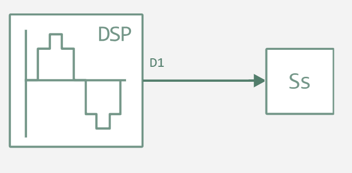
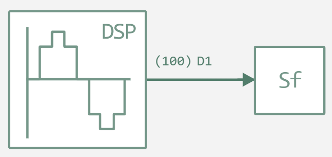
To demonstrate, let's take two identical models with identical parameters. There is one difference: in the first case, pipeline calculations will be used, and in the second, vector calculations.
The models themselves are shown in the figure below.
Function for launching the model
Pkg.add(["TickTock"])
# Enabling the auxiliary model launch function.
function run_model( name_model)

    Path = (@__DIR__) * "/" * name_model * ".engee"

    if name_model in [m.name for m in engee.get_all_models()] # Checking the condition for loading a model into the kernel
        model = engee.open( name_model ) # Open the model
        model_output = engee.run( model, verbose=true ); # Launch the model
    else
        model = engee.load( Path, force=true ) # Upload a model
        model_output = engee.run( model, verbose=true ); # Launch the model
        engee.close( name_model, force=true ); # Close the model
    end
    sleep(5)
    return model_output
end
Comparison of work speed
Now let's move on to comparing the speed of work. Let's use the TickTock library and tick() functions. and tok()
tick() — records the current time. It is usually used to start measuring time.
tok() — calculates and outputs the time elapsed since the last tick() call.
Features and benefits of using TickTock:
- Functions of tick() and tok() Provide a simple and intuitive way to measure time without having to manually calculate the difference between start and end times.
- TickTock works with high time accuracy, which allows you to get reliable data on the duration of code execution, even for very fast operations.
- The measurement result is displayed in an easy-to-read format (seconds, milliseconds), as well as the standard Float64 output data format, which makes it easy to convert these values to minutes or hours.
using TickTock
tick()
run_model("sin_Sample") # Launching the model.
Ts = tok()
tick()
run_model("sin_Frame") # Launching the model.
Tf = tok()
println("Time sin_Sample: $(Ts)")
println("Time sin_Frame: $(Tf)")
println("Time difference: $(abs(Ts-Tf))")
As we can see from the calculation of the difference, the execution time differs slightly. Let's also compare the simulation results in order to make sure that the models are identical.
Ss = collect(Ss);
Sf = collect(Sf);
Sf = reduce(vcat, Sf.value)

println("Size sin_Sample: $(size(Ss))")
println("Size sin_Frame: $(size(Ss))")
As we can see, the dimensions of the signals are equal.
gr()
error = abs.(Sf[1:100]-Ss.value[1:100]);

plot(Ss.value[1:100], label="sin_Sample")
plot!(Sf[1:100], label="sin_Frame")
plot!(error, label="difference")
title!("sum_error: $(sum(error))")
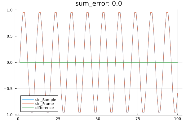
The signals are identical both in size and in comparison of the signals themselves.
Conclusion
In this example, we looked at how the TickTock library can be used to compare the speed of different models. This tool is useful for analyzing the performance of your models and evaluating the need to optimize them.