We study solvers with variable pitch
In this example, we will analyze how the choice of a solver affects the calculation of the trajectory of the Foucault pendulum using a mathematical model. We will demonstrate the work of the solvers DP5 and Tsit5 (ode45), Rodas4 (ode15s), BS3 (ode23) and Trapezoid (ode23t). The names of similar solvers adopted in Simulink are given in parentheses.
The solution of the problem will be given in the form of differential equations having the features of a rigid system. Explicit integration methods (using data from pairs of neighboring points to find the derivative) are poorly suited for such systems. An incomparably better result is usually given by implicit methods that find a solution based on the data of several neighboring points from the desired one. The definition of rigid systems is rather vague, but there is one common feature of their behavior – they may require a very small integration step, without which calculations are unstable (for example, the result goes to infinity).
Rigidity is often inherent in systems of equations consisting of two components, the state of which changes at different rates: very fast and very slow.
Foucault's Pendulum
Foucault's pendulum model is an example of a rigid system. The pendulum oscillates once every few seconds (* a rapidly changing component*), but it is also affected by the rotation of the Earth (* a slowly changing component*), the frequency of which is calculated in days, years, etc. The movement of the pendulum is dictated by inertia and gravity. And the plane in which the oscillations occur rotates synchronously with the daily rotation of the Earth.
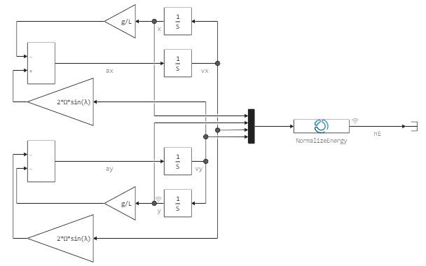
Let's define the model through two differential equations that describe the motion of the load at the end of the pendulum in the x-y plane (top view). We will evaluate the work of different solvers by studying the law of conservation of the total energy of the system.
The model does not take into account friction and air resistance, so the equations of motion look very concise.:
where – the angular velocity of the Earth's rotation around the axis, – geographical latitude, – acceleration of free fall, and – coordinates of the center of mass of the load at the end of the pendulum.
Pkg.add(["Measures", "Serialization"])
using Plots
gr( fmt=:png )

# Model parameters and initial conditions
Ω = 2*pi/86400;    # Angular velocity of the Earth's rotation around its axis (rad/s)
λ = 59.93/180*pi;  # Latitude (rad)
g = 9.8195;        # Acceleration of gravity (m/s^2)
L = 97;            # Length of the pendulum (m)

initial_x = L/100; # The initial value of the x (m) coordinate
initial_y = 0;     # The initial value of the y coordinate (m)
initial_xdot = 0;  # Initial value of the x-axis velocity (m/s)
initial_ydot = 0;  # Initial value of the y-axis velocity (m/s)

TotalEnergy = 1/2*(initial_xdot^2 + initial_ydot^2) + g*(L-sqrt( L^2-initial_x^2-initial_y^2));
The model that implements these equations is shown below.:
Variable-pitch solvers
We are going to compare the following integrators (solvers):
| Name (Julia) | Name (Simulink) | Type of tasks | Accuracy | When to use it |
|---|---|---|---|---|
| DP5, but better Tsit5 | ode45 |
Not rigid | Average | By default. Try it first |
| BS3 | ode23 |
Not rigid | Low | If large errors are allowed in the task or for medium-hard systems |
| VCABM, but better Vern7 | ode113 |
Not rigid | From low to high | Low error, suitable for high-volume computing tasks |
| QNDF, FBDF, but better Rodas4, KenCarp4, TRBDF2, RadauIIA5 | ode15s |
Tough ones | From low to medium | If ode45 it works too slowly due to the rigidity of the task. |
| Rosenbrock23, but better Rodas4 | ode23s |
Tough ones | Low | With low accuracy requirements for solving difficult problems and with a constant matrix масс |
| Trapezoid | ode23t |
Moderately hard | Low | For moderately harsh tasks, if a solution without numerical damping is needed. |
| TRBDF2 | ode23tb |
Tough ones | Low | With low requirements for the accuracy of the solution, for solving tough tasks |
If you don't find the right solver when solving problems, and you're more familiar with the names of Simulink solvers, pay attention to the comparison from [this article](https://docs.sciml.ai/DiffEqDocs/stable/solvers/ode_solve /). Engee mainly uses the names of solvers accepted in Julia packages.
Comparison criteria
The quality of the solution of each integration algorithm can be assessed in several ways. First, if the problem has an analytical solution, then you can compare the result of numerical integration with the theoretical result. You can also estimate the time it takes for an algorithm to solve a problem and use the time cost as a basis for comparison.
Unfortunately, there is no exact analytical solution for Foucault's pendulum, and the approximate ones have their own inherent errors.
Saving the total energy of the system
We will evaluate the quality of each solver's solution by checking compliance with the law of conservation of energy in the system.
In the absence of friction, the total energy of the pendulum must remain constant. Numerical solutions will not show us the ideal conservation of energy due to the accumulation of errors.
So, in the example, we will calculate the total energy of the system at each integration step. Ideally, the total energy should not change at all and the difference should be zero. Total energy is the sum of potential and kinetic energy. This is exactly the value that the block calculates. NormalizeEnergy:
where – total energy at the initial moment of time.
The change in the total energy from the moment of the beginning to the end of the calculations will allow us to evaluate the quality of the numerical solution.
modelName = "foucault_pendulum_model"
model = modelName in [m.name for m in engee.get_all_models()] ? engee.open( modelName ) : engee.load( "$(@__DIR__)/$modelName.engee" );

engee.set_param!( modelName, "SolverName"=>"BS3", "RelTol"=>1e-5 ) # Let's install a solver similar to ode23
dt_ode23 = @elapsed begin x_ode23 = engee.run( modelName ); end;

engee.set_param!( modelName, "SolverName"=>"Trapezoid", "RelTol"=>1e-5 ) # Let's install a solver similar to ode23t
dt_ode23t = @elapsed begin x_ode23t = engee.run( modelName ); end;
Let's compare two integrators by this parameter.:
- BS3 (
ode23) is a rather crude algorithm unsuitable for rigid systems, - Trapezoid (
ode23t) is also a rather crude algorithm, but it is suitable for rigid systems.
using Plots

plot( x_ode23["nE"].time, x_ode23["nE"].value, label="ode23", title="Comparison of the quality of solutions at RelTol = 1e-5", lw=2 )
plot!( x_ode23t["nE"].time, x_ode23t["nE"].value, ylimits=(0,1.1), label="ode23t", leg=:bottomleft, lw=2 )
plot!( xlabel="Time (s)", ylabel="Relative total energy",
       titlefont=11, guidefontsize=10, tickfontsize=9, legendfontsize=10 )
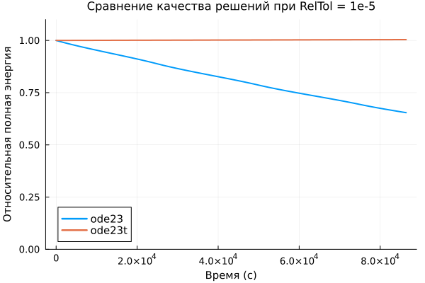
As it is easy to see, the "losses" of total energy associated with inaccuracies in the integrator are almost imperceptible in the first case, and about 20% per day in the second case.
As the total energy of the pendulum decreases, the oscillation amplitude decreases, as we will see by plotting the following graphs. We will also see that the plane of oscillation of the pendulum changes with time (unfolds).
using Measures

bar_w = 150 # The "thickness" of the lines fixing the plane of oscillation of the pendulum at different moments

lastPlane_y = maximum( x_ode23["y"].value[end-bar_w:end] )
lastPlane_x = maximum( x_ode23["x"].value[end-bar_w:end] )
plot( x_ode23["x"].value[1:2:end], x_ode23["y"].value[1:2:end],
      st=:scatter, ms=.8, markerstrokecolor=:blue, markercolor=:blue,
      title="The position of the load of the Foucault pendulum (top view)\rEcipient: ode23; RelTol = 1e-5; Execution time=$(round(dt_ode23,digits=2)) with",
      titlefont=9, guidefontsize=8, tickfontsize=8, leg=:none, xlabel="X-coordinate (m)", ylabel="Y coordinate (m)",
      left_margin=13mm, bottom_margin=13mm, top_margin=5mm, aspect_ratio = :equal )
scatter!( [initial_x], [0], mc=:black, ms=8 )                                                # The Black Ball
plot!( x_ode23["x"].value[1:bar_w], x_ode23["y"].value[1:bar_w], lc=:black, lw=3 )           # The black line
plot!( x_ode23["x"].value[end-bar_w:end], x_ode23["y"].value[end-bar_w:end], lc=:red, lw=3 )

vlen = length(x_ode23["x"].value)
half_vec = ceil(Int32, vlen/2);
plot!( x_ode23["x"].value[(half_vec-bar_w):half_vec], x_ode23["y"].value[(half_vec-bar_w):half_vec], lc=:yellow, lw=3 )

annotate!( initial_x, 0.05, text("Starting position", :black, rotation = 90, 7, :left) )
plot!( [lastPlane_x-0.1, lastPlane_x-0.8], [lastPlane_y, lastPlane_y], lw=13, lc=:white ) # The white line
p1 = annotate!( lastPlane_x-0.1, lastPlane_y, text("The final plane", :red, 7, :right) )

plot( x_ode23t["x"].value[1:2:end], x_ode23t["y"].value[1:2:end], st=:scatter, ms=.8, markerstrokecolor=:blue, markercolor=:blue,
          title="The position of the load of the Foucault pendulum (top view)\rEcipient: ode23t; RelTol = 1e-5; Execution time=$(round(dt_ode23t,digits=2)) with",
          titlefont=9, guidefontsize=8, tickfontsize=8, leg=:none, xlabel="X-coordinate (m)", ylabel="Y coordinate (m)",
          left_margin=13mm, bottom_margin=13mm, top_margin=5mm, aspect_ratio = :equal )
plot!( x_ode23t["x"].value[1:bar_w], x_ode23t["y"].value[1:bar_w], lc=:black, lw=3 )           # The black line
plot!( x_ode23t["x"].value[end-bar_w:end], x_ode23t["y"].value[end-bar_w:end], lc=:red, lw=3 )

vlen = length(x_ode23t["x"].value)
half_vec = ceil(Int32, vlen/2);
plot!( x_ode23t["x"].value[(half_vec-bar_w):half_vec], x_ode23t["y"].value[(half_vec-bar_w):half_vec], lc=:yellow, lw=3 )

p2 = plot!( [initial_x], [0], mc=:black, st=:scatter, ms=8 )

plot( p1, p2, size = (1000,450) )
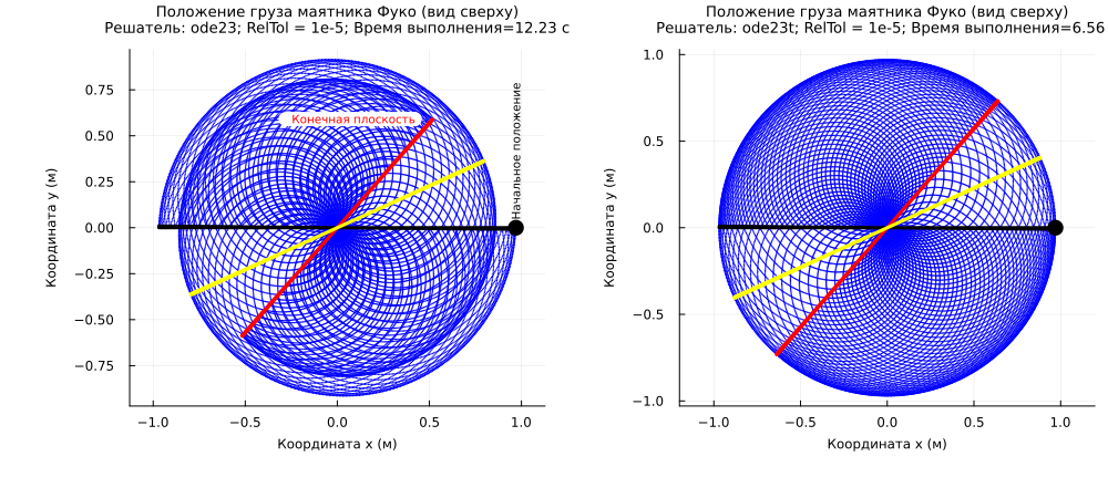
We have observed how the quality of the solution for rigid and non-rigid systems depends on the choice of a solver. The plane in which the pendulum oscillates does not make a complete turn during the day: the angle of rotation depends on the geographical latitude.
Let's build a graph that will allow us to study in detail the speed and quality of work of different solvers on the Foucault pendulum simulation problem. We will compare the results for different numerical integration methods and see how the energy of the system is conserved at different relative error values.
It may take several minutes to execute this script, so to save time when running the script again, you have the option to download data from a previously saved file. results.bin.
using Serialization

# To update the results, delete the "results" file
if !isfile( "$(@__DIR__)/results.bin" )

    solvers = ["Tsit5" "DP5" "Rosenbrock23" "Trapezoid" "BS3"]
    reltols = 10 .^( collect(range(-7,-3,length=9)) )

    nE_results = zeros( length(solvers), length(reltols) )
    dt_results = zeros( length(solvers), length(reltols) )

    # Let's study all the combinations (solver; relative accuracy)
    for (i,solver) in enumerate(solvers)
        print( solver, ": ")
        for (j,reltol) in enumerate(reltols)
            print( round(reltol, sigdigits=3), ", " )
            # Let's set a new solver and relative accuracy for the model.
            engee.set_param!( modelName, "SolverName"=>solver, "RelTol"=>reltol )
            # We calculate the model and measure the time at the same time
            dt_results[i,j] = @elapsed begin sim_data = engee.run( modelName ); end;
            # Calculating the ratio
            nE_results[i,j] = abs( sim_data["nE"].value[1] - sim_data["nE"].value[end] )
        end
        println()
    end

    serialize( "$(@__DIR__)/results.bin", (solvers, reltols, nE_results, dt_results) )
else
    (solvers, reltols, nE_results, dt_results) = deserialize( "$(@__DIR__)/results.bin" );
end
Now we can build and analyze the graph.
markerShapes_ = [ :circle :rect :star5 :diamond :hexagon ]
markerStrokeColors_ = [1 2 3 4 5]

plot(
      plot( reltols, nE_results', xscale=:log10, yscale=:log10,
            label=solvers, ylabel="Max. relative power output",
            titlefont=11, guidefontsize=8, tickfontsize=9, legendfontsize=7, left_margin=13mm, legend=:bottomleft,
            marker=markerShapes_, markerstrokecolor=markerStrokeColors_, markercolor=RGBA(1,1,1,0) ),
      plot( reltols, dt_results', xscale=:log10,
            label=solvers, ylabel="Execution time\nmodels (s)", xlabel="Relative accuracy of the numerical integration algorithm",
            titlefont=11, guidefontsize=8, tickfontsize=9, legendfontsize=7, left_margin=13mm, bottom_margin=13mm,
            marker=markerShapes_, markerstrokecolor=markerStrokeColors_, markercolor=RGBA(1,1,1,0) ),
      size=(800,500),
      layout=(2,1)
    )
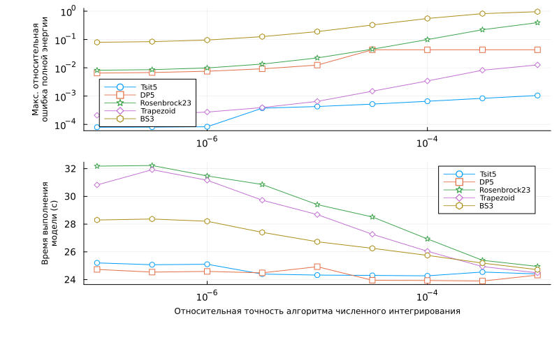
We see a zone where the criterion of under-forecasting the total energy of the system practically ceases to change (at relative_tolerance < 1e-6).
This is due to the behavior of a particular model. But, in general, it is worth considering that a decrease in the relative accuracy of the solver does not necessarily lead to an increase in accuracy. When we set the desired accuracy limit for the solution and choose other solver settings, we should always think about the acceptable time spent on simulation.
We are most likely satisfied with the accuracy of estimating the position of the load at the end of the pendulum by a few centimeters. And it is no longer advisable to perform calculations with an accuracy of microns, since it will be very difficult to conduct an equally accurate real experiment to validate the model.
Conclusion
We have studied how the choice of a numerical method for solving the equations of a system (the choice of a solver) affects the results and course of solving a rigid system. A lot depends on the solver: after all, the algorithm should not only allow us to achieve the desired accuracy of the solution, but also be completed in a reasonable time.
The relative accuracy of the variable-step solver (as well as the integration step of the constant-step solver) should be small enough so that the solution does not become unstable.
All solvers have their advantages and disadvantages, but some obviously work better when solving tough problems. And variable-step solvers are generally more stable than constant-step solvers.