Hydraulic system simulation
This example will demonstrate the simulation of a hydraulic cylinder assembled from the blocks of the basic library.
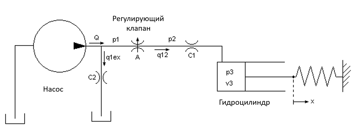
The figure shows a schematic diagram of the model. The pump model directs the flow , forming pressure , under the action of which the laminar flow it flows out on release. The control valve simulates a turbulent flow through a variable-area orifice. This thread, , generates an intermediate pressure, , which undergoes a subsequent drop in the line connecting it to the drive cylinder. Cylinder pressure, , moves the piston, which is under the action of force from the spring, as a result of which it is in the x position.
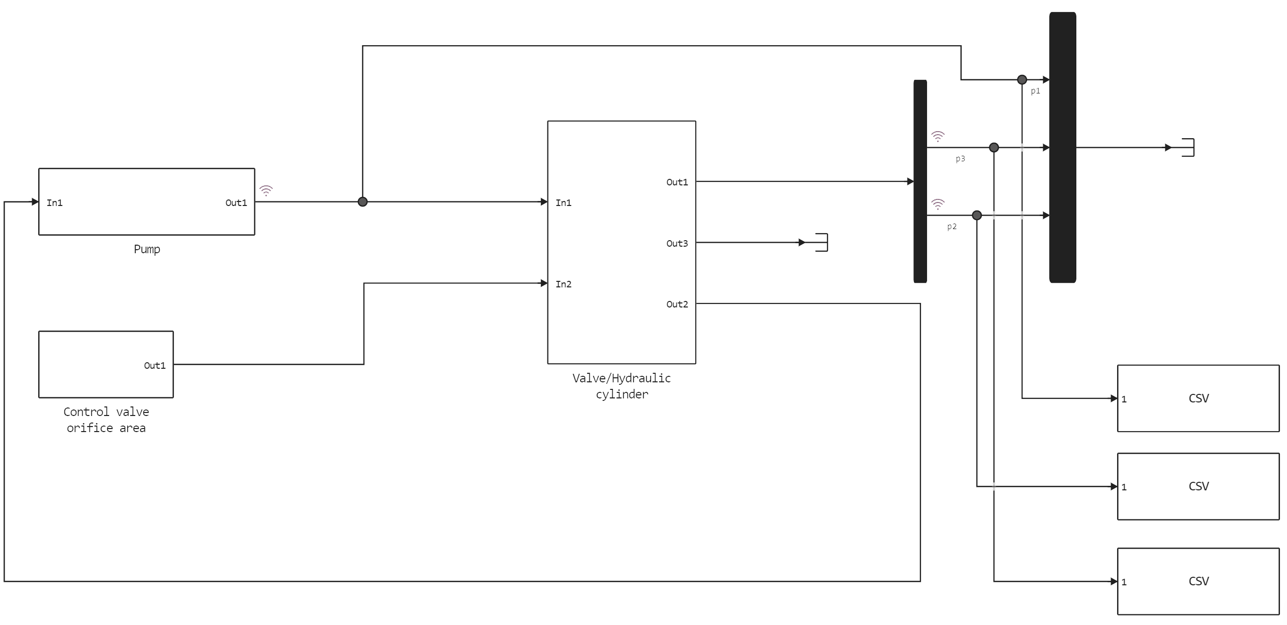
Model diagram in Engee:
At the pump outlet, the flow is divided into two components: the leakage flow and the flow to the control valve. We are simulating a leak, , as a laminar flow (see equation block 1).
Pkg.add(["CSV"])
cd( @__DIR__ ) # Let's move to the directory where the current script is located.
homePath = string(@__DIR__)
Equation block 1
where:
- - pump flow
- - flow to the control valve
- - leakage current
- - flow coefficient
A turbulent flow through a control valve is simulated. Function and the module allows you to take into account the flow in both directions (see equation block 2).
Equation block 2
where:
- - flow through the control valve
- - the flow rate through the hole
- - the area of the hole
- - pressure after the control valve
- - density of the liquid
The fluid pressure in the cylinder increases due to this flow. The compressibility of the liquid was also modeled (see equation block 3).
Equation block 3
where:
- - volume of liquid at pressure ,
- - the rate of pressure change in the cylinder over time,
- - volumetric modulus of elasticity of a liquid,
- - the volume of liquid in the piston at ,
- - the cross-sectional area of the cylinder
The piston and spring weights were not taken into account due to the high hydraulic forces. Equation block 4 calculates the balance of forces on the piston.
Equation block 4
where:
- - stiffness of the spring
- - laminar flow coefficient
The "Pump" subsystem
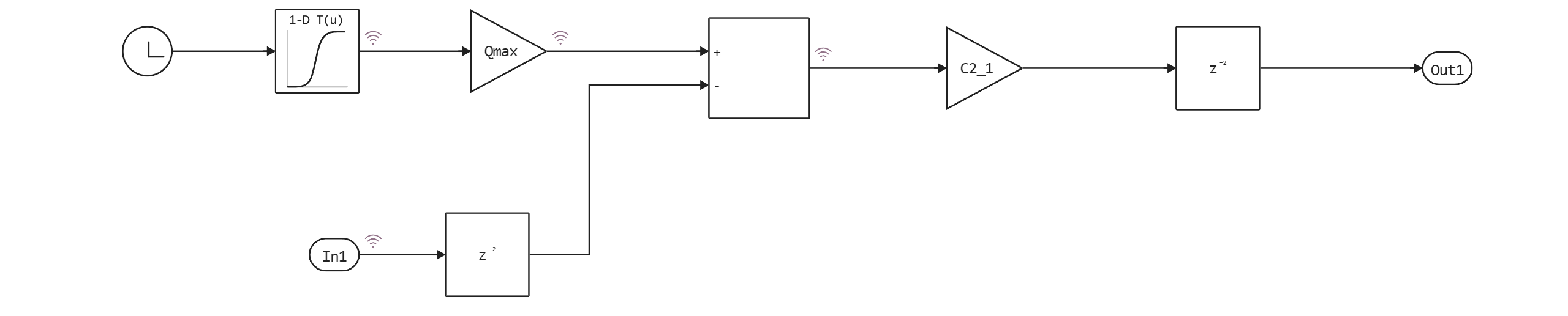
Double-click on the subsystem named "Pump" to open the pump model. It calculates the supply pressure depending on the flow rate of the pump itself and the flow rate of the system elements after it. The one-dimensional table defines the consumption data depending on the time. The model calculates the pressure as indicated in equation block 1. Because is a direct function of (through the control valve), an algebraic loop is formed. Setting the initial pressure value, , allows you to get a more efficient solution.
The "Valve/Hydraulic cylinder" subsystem
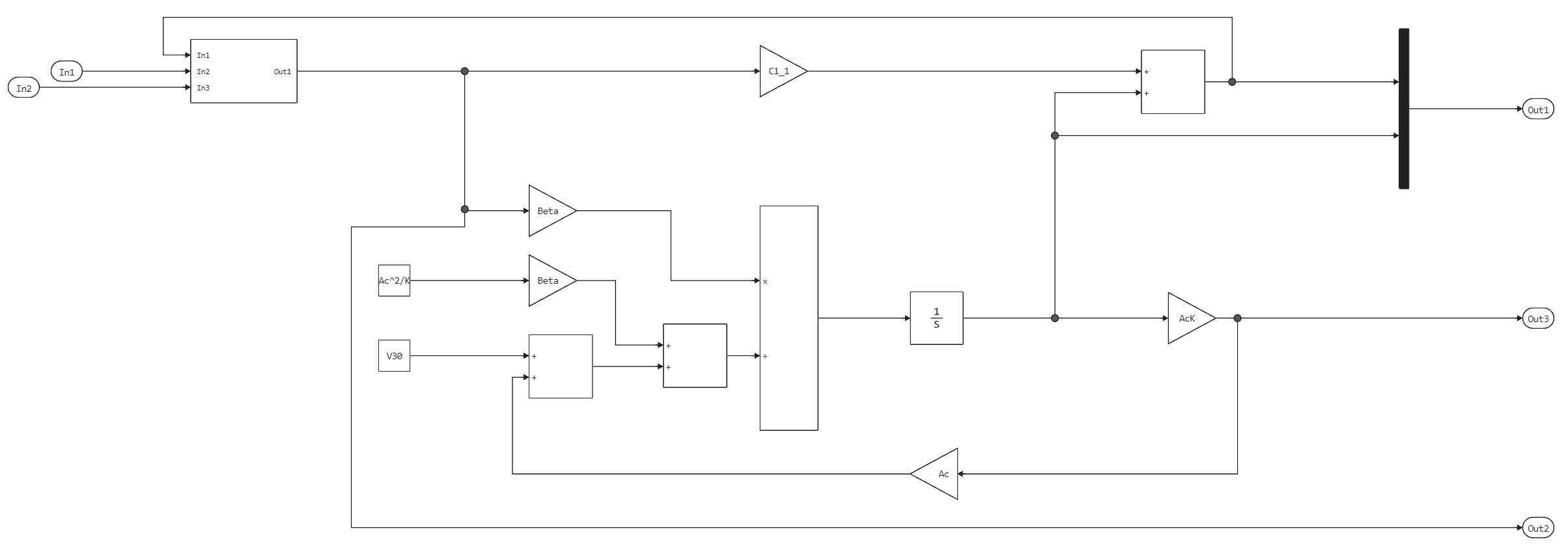
Double-click on the subsystem named "Valve/Hydraulic cylinder" to open the models of the control valve and hydraulic cylinder. A system of differential algebraic equations simulates pressure increase in a cylinder using pressure , which appears as a derivative in equation block 3. If we neglect the mass of the piston, then its position and spring force will be directly proportional , and the speed is directly proportional to the time derivative of . Intermediate pressure is the sum of and the pressure drop caused by the flow from the valve to the cylinder (equation block 4).
The subsystem of the control valve calculates the flow through the hole (equation block 2). It uses pressure at the inlet and outlet of the hole and a variable area as input data.
Determination of hydraulic system parameters and initial conditions:
The system parameters and initial conditions are set in the code cell:
A = 0.01
Ac = 0.001
Beta = 700000000
C1 = 2.50000000000000e-08
C2 = 3.00000000000000e-09
Cd = 0.610000000000000
F20 = 0
I = 100
K = 20500
V30 = 2.000000000000000e-05
V2 = 1.250000000000000e-05
V1 = 1.250000000000000e-05
rho = 800
Qmax = 0.005000000000000
p10 = 4.166666666666667e+06
M = 2500
m = 1.000000000000000e-03
L = 1.500000000000000
KA = 0.030000000000000;
Cdsqrt = Cd*sqrt(2/rho);
AcK = Ac/K
C1_1 = 1/C1
C2_1 = 1/C2
Ac2K = Ac^2/K;
Sample_Time = 0.0001;
The code cell must be executed before starting the simulation.
Launching and loading the model:
In this code cell, methods are used to interact with the control flow of the program, try/catch:
try
    engee.close("single_hydraulic_cylinder_simulation", force=true) # closing the model
    catch err # if there is no model to close and engee.close() is not executed, it will be loaded after catch.
        m = engee.load("$(@__DIR__)/single_hydraulic_cylinder_simulation.engee") # loading the model
    end;
try
    engee.run(m, verbose=true) # launching the model
    catch err # if the model is not loaded and engee.run() is not executed, the bottom two lines after catch will be executed.
        m = engee.load("$(@__DIR__)/single_hydraulic_cylinder_simulation.engee") # loading the model
        engee.run(m, verbose=true) # launching the model
    end
Loading and visualizing the data obtained during the simulation.
Reading csv files with data on pressure changes in different parts of the hydraulic system,
followed by conversion to a dataframe and matrix:
using DataFrames, Plots, CSV # connecting libraries
p1 = Matrix(CSV.read("p1.csv", DataFrame)); # uploading data on pressure changes at the pump outlet
p2 = Matrix(CSV.read("p2.csv", DataFrame)); # uploading pressure change data after the control valve
p3 = Matrix(CSV.read("p3.csv", DataFrame)); # loading data on pressure changes in the cylinder
Enabling a backend graphics display method:
plotlyjs()
Plotting a graph describing pressure changes in sections of the hydraulic system:
plot(p1[:,1], p1[:,2], label="Pressure change at the pump outlet")
plot!(p2[:,1], p2[:,2], label="Pressure change after the control valve")
plot!(p3[:,1], p3[:,2], label="Cylinder pressure change")
At the beginning of the simulation, the control valve has a zero opening area, which then increases to sq.m. during the entire simulation lasting 0.1 seconds. When the valve is closed, the entire pump flow becomes a leak.
When the valve opens, the pressure and they increase, while it decreases in response to an increase in consumption. When the pump flow stops, the spring and piston act as a hydraulic accumulator, and it is continuously decreasing. The behavior changes as the flow from the pump is restored.
Conclusion:
In this example, a simulation of a hydraulic system assembled from a library of basic blocks was demonstrated. The simulation data was loaded, preprocessed, and visualized using the functions of the invoked libraries.