Analysis of the spring damper system
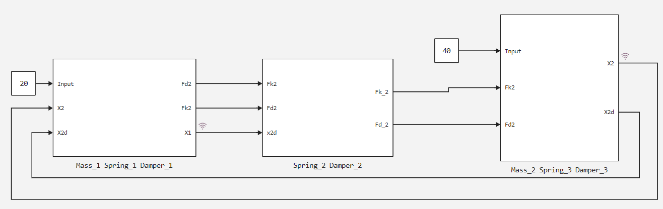
The system diagram is shown in the figure below.
The implementation will include three subsystems:
- mass-1, spring-1, dumper-1.
- spring-2, dumper-2.
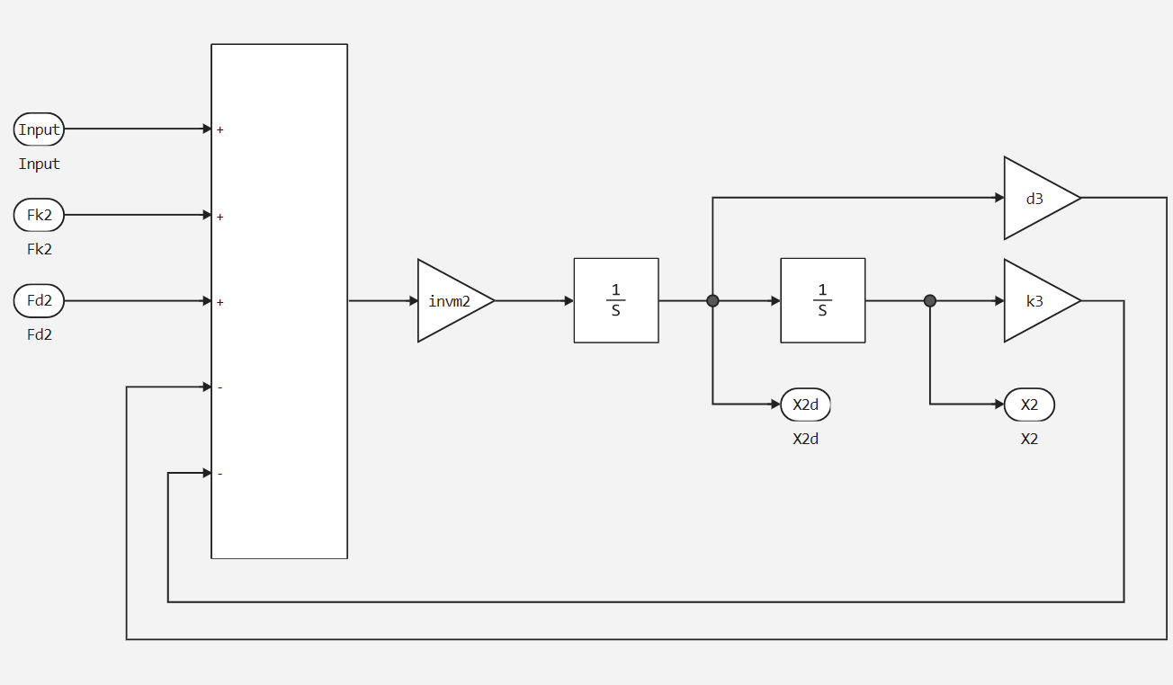
- Mass-2, spring-3, dumper-3.
The figure below shows the upper level of the implemented system.
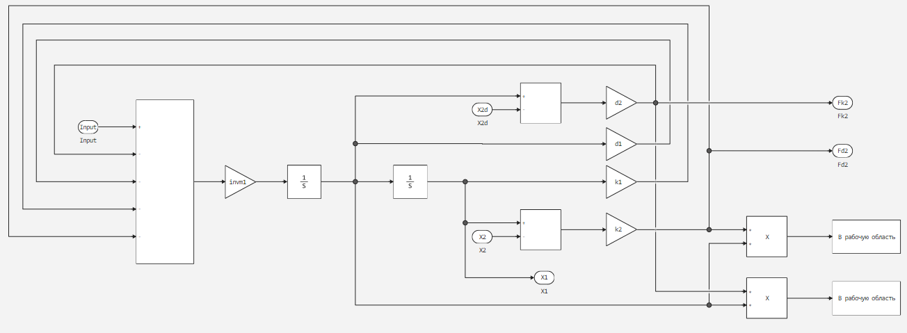
The contents of all the subsystems of the model are also shown below in their chronological order. The first one is Mass_1 Spring_1 Damper_1.
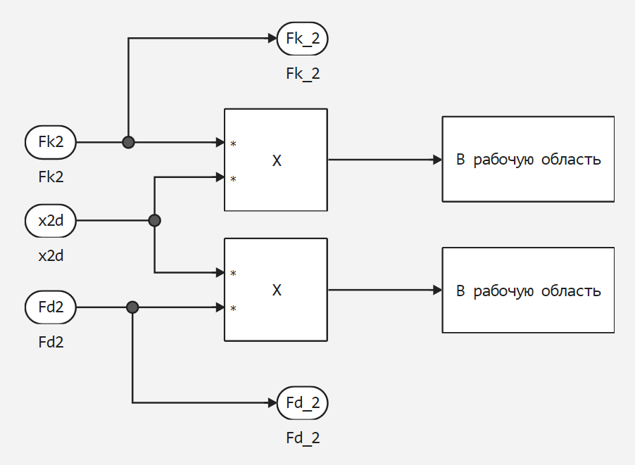
The second one is Spring_2 Damper_2.
And the third is Mass_2 Spring_3 Damper_3.
Now let's move on to declaring the parameters of these systems.
# Determination of body masses
m1 = 20;
m2 = 10;

# Calculating the inverse fraction of the mass of bodies
invm1 = 1/m1;
invm2 = 1/m2;

# Determination of damping coefficients
d1 = 0.5;
d2 = 0.2;
d3 = 2;

# Spring elasticity coefficients
k1 = 5;
k2 = 3;
k3 = 2;

# Initial states of integrators for the first and third subsystems
init_integrator_1 = 0.0001;
init_integrator_3 = 0;

# Input impact forces
F1 = 20;
F2 = 40;
Let's run the model with our parameters.
function run_model( name_model, path_to_folder )

    Path = path_to_folder * "/" * name_model * ".engee"

    if name_model in [m.name for m in engee.get_all_models()] # Checking the condition for loading a model into the kernel
        model = engee.open( name_model ) # Open the model
        model_output = engee.run( model, verbose=true ); # Launch the model
    else
        model = engee.load( Path, force=true ) # Upload a model
        model_output = engee.run( model, verbose=true ); # Launch the model
        engee.close( name_model, force=true ); # Close the model
    end

    return model_output
end
run_model( "PowerAnalysis", @__DIR__ )
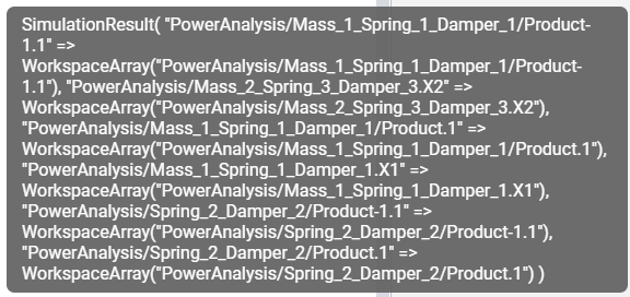
In this demonstration, the output signals describing the oscillatory processes of the masses are logged not through To Workspace, but through bus logging. Therefore, when running the model, we see that several variables have been created with the name of the subsystem and the name of the output port, which are stored in the simout structure. If more than four signals are logged during the simulation, all their names can be viewed by hovering the cursor over the simout variable.
.png)
# Reading of encoded signals from simout
X1 = simout["PowerAnalysis/Mass_1_Spring_1_Damper_1.X1"];
X1 = collect(X1);
X2 = simout["PowerAnalysis/Mass_2_Spring_3_Damper_3.X2"];
X2 = collect(X2);
X1[1:3,:]
As we see the data reading field, from simout we get a DataFrames structure containing timestamp and data fields. We get a similar structure when reading WorkspaceArray.
Now let's build a comparative graph of the oscillations of the two bodies from our model. In this case, from the sum of the impact forces in relation to body weight, we get acceleration.
Then, by integrating, we calculate the speed. And due to the second integration, we get a move, which in turn we log.
using Plots # Enabling the charting library
plotly()
plot(X1.time,X1.value) # The first body
plot!(X2.time,X2.value) # The second body
As we can see from the graph, the fluctuations of the first body are more intense than the second. This is primarily due to the fact that the mass of the first body is twice the mass of the second body.
Also, during the simulation, we logged the power of the dampers and springs. Let's analyze this data.
Power is calculated through the product of force and speed.
# The damper
Fd2x1d = simout["PowerAnalysis/Mass_1_Spring_1_Damper_1/Product.1"];
Fd2x1d = collect(Fd2x1d);
Let's build a graph.
plot( Fd2x1d.time, Fd2x1d.value )
In these two graphs, we see the power differences for the first spring and the first damper.
Conclusion
In this demonstration, we analyzed the behavior of the damper system, as well as considered various possibilities for logging signals from models in Engee.