Subsystems
The purpose of this demonstration is to show how to use all kinds of subsystems implemented in Engee. To do this, let's look at a few simple models.
using Plots # Library for rendering simulation results

# Enabling the auxiliary model launch function.
function run_model( name_model, path_to_folder )

    Path = path_to_folder * "/" * name_model * ".engee"

    if name_model in [m.name for m in engee.get_all_models()] # Checking the condition for loading a model into the kernel
        model = engee.open( name_model ) # Open the model
        model_output = engee.run( model, verbose=true ); # Launch the model
    else
        model = engee.load( Path, force=true ) # Upload a model
        model_output = engee.run( model, verbose=true ); # Launch the model
        engee.close( name_model, force=true ); # Close the model
    end

    return model_output
end

# The path to the folder with models
path = "$(@__DIR__)/models"
Enabled Subsystem
The first subsystem option that we will consider in this example is Enabled Subsystem. We are talking about a conditionally executed subsystem that is started once at each main time step, as long as the control signal has a positive value. If the signal crosses zero during a smaller time step, the subsystem does not turn on or off until the next major time step.
The control signal can be a scalar or a vector.
- If the scalar value is greater than zero, the subsystem is executed.
- If any of the values of the vector element is greater than zero, the subsystem is executed.
To use this functionality, add a block to the Subsystem block or to the root level of the model referenced by the Model block. If you are using Enable at the root level of the model, follow these steps.
- For multi-speed models, set the solver to single-task mode.
- For models with a fixed step size, at least one block in the model must operate at a specified speed of a fixed step size.
The picture below is an illustration of this example.
In this example, the control signal is a sine wave, and the input signal is a counter.
run_model("enabled_subsystem",path) # Launching the model.
# Reading of encoded signals from simout
data1 = simout["enabled_subsystem/SubSystem.Out1"];
data1 = collect(data1);
en1 = simout["enabled_subsystem/Sine Wave.1"];
en1 = collect(en1);
Let's plot the dependence of the output data on the control signal.
plot(data1.time,data1.value)
plot!(en1.time,en1.value)
As we can see from the graph, at those moments when the control signal drops below 0, the output signal fades.
Action Subsystem
Action Port controls the subsystem execution. The block adds an external input port for action signals to the subsystem. The action signal controls the signal connected to the Action port of the Subsystem block.
Used in models containing blocks:
- If
.png)
- Switch Case
Let's run these two models and analyze the results. Let's start with the cif model.
run_model("if_subsystem",path) # Launching the model.
# Reading of encoded signals from simout
SysOutput_1 = simout["if_subsystem/SysOutput_1"];
SysOutput_1 = collect(SysOutput_1);
SysOutput_2 = simout["if_subsystem/SysOutput_2"];
SysOutput_2 = collect(SysOutput_2);
plot(SysOutput_1.time,SysOutput_1.value)
plot!(SysOutput_2.time,SysOutput_2.value)
As we can see, in the case of if, the input sinusoid was divided into two signals: according to the condition greater than 0 and less than 0.
run_model("switch_case_subsystem",path) # Launching the model.
# Reading of encoded signals from simout
SysOutput_1 = simout["switch_case_subsystem/SysOutput_1"];
SysOutput_1 = collect(SysOutput_1);
SysOutput_2 = simout["switch_case_subsystem/SysOutput_2"];
SysOutput_2 = collect(SysOutput_2);
En = simout["switch_case_subsystem/Pulse Generator.1"];
En = collect(En);
Let's plot the dependence of the output signals on the control signal.
plot(SysOutput_1.time,SysOutput_1.value)
plot!(SysOutput_2.time,SysOutput_2.value)
plot!(En.time,En.value)
As we can see, when the control signal is 1, the data is written from the upper subsystem. If the data is 0, then we get a graph of data from the second subsystem. Otherwise, the output signal on the subsystem freezes while waiting for the control signal.
Triggered Subsystem
Unlike the Enabled Subsystem block, the Triggered Subsystem block always keeps its output parameters at the last value between triggers. In addition, running subsystems cannot reset block states during execution; the states of any discrete block are saved between triggers.
The Trigger block adds an external signal to control subsystem execution. The subsystem will be executed once at each step when the value of the control signal is changed in the specified way. The block icon changes depending on the value selected for the Trigger type parameter. In addition, the Trigger block can be added to Enable. In this section, we will analyze both applications of the Triggered Subsystem.
To begin with, let's look at an example of a simple Triggered Subsystem. The implementation of the model using this approach is shown in the figure below.
.png)
run_model("triggered_subsystem",path) # Launching the model.
# Reading of encoded signals from simout
SysOutput_1 = simout["triggered_subsystem/SubSystem.Out1"];
SysOutput_1 = collect(SysOutput_1);
En = simout["triggered_subsystem/Sine Wave-1.1"];
En = collect(En);
plot(SysOutput_1.time,SysOutput_1.value)
plot!(En.time,En.value)
According to the resulting data, we can see that such a subsystem is triggered only at the moment when the sinusoid 0 intersects.
Now let's consider the use of the Trigger and Enable blocks in the same subsystem. The figure below shows the model we implemented.
run_model("triggered_enabled_subsystem",path) # Launching the model.
# Reading of encoded signals from simout
Data = simout["triggered_enabled_subsystem/SubSystem.Out1"];
Data = collect(Data);
Trigger = simout["triggered_enabled_subsystem/Trigger.1"];
Trigger = collect(Trigger);
Enable = simout["triggered_enabled_subsystem/Enable.1"];
Enable = collect(Enable);
Let's analyze the output relative to the two control signals.
plot(Data.time,Data.value)
plot!(Trigger.time,Trigger.value)
plot!(Enable.time,Enable.value)
As we can see, the frequency of the Enable signal is three times higher than the frequency of the Trigger, so these two signals intersected only once and thus started the subsystem.
For Each Subsystem
The For Each block is a control block for For Each Subsystem. This subsystem allows you to process parts of the input signals.
Each block within this subsystem maintains a separate set of states for each element or subarray that it processes. As a set of subsystem blocks processes elements or subarrays, the subsystem combines the results to form output signals.
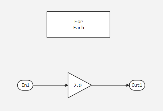
The figures below show the model in which the For Each block is used.
.png)
.png)
run_model("for_each_model1",path) # Launching the model.
# Reading of encoded signals from simout
Data_in = simout["for_each_model1/Constant.1"];
Data_in = collect(Data_in);
Data_out = simout["for_each_model1/SysOutput_1"];
Data_out = collect(Data_out);
print(string(Data_in.value[1]) *" --> " * string(Data_out.value[1]))
As we can see, the result was a piecemeal multiplication of the input data by 2.
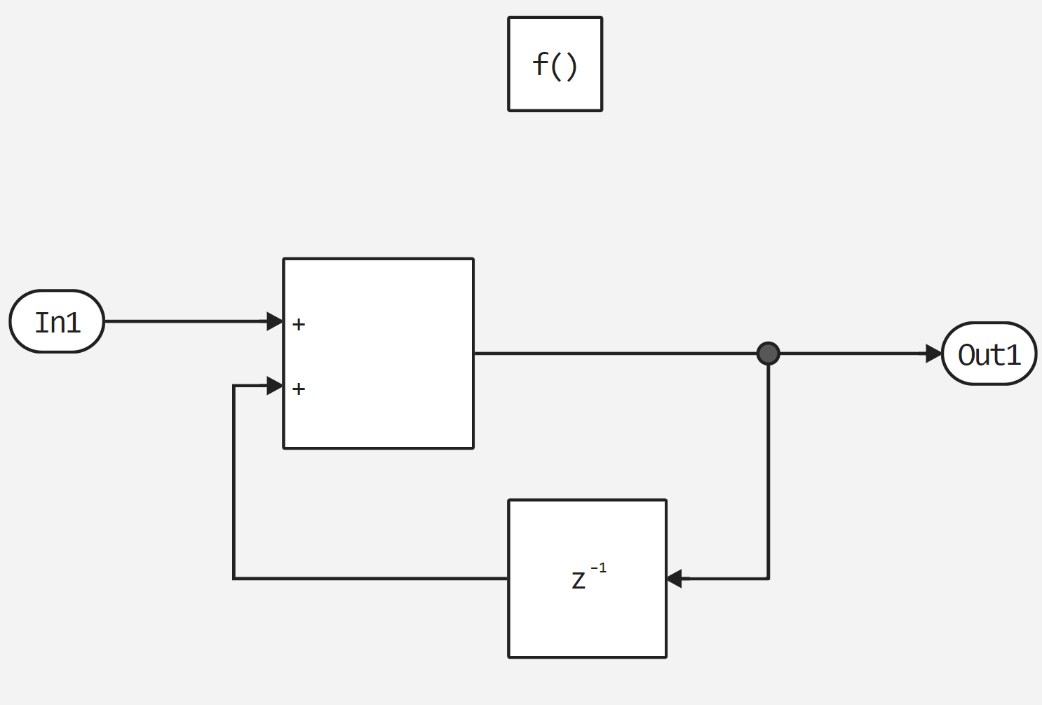
This block also allows you to create indexes for input data and output them as a port. The figures below show such an application For Each.
.png)
.png)
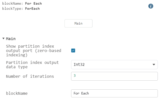
The counter settings also indicate that the number of iterations is 3.
run_model("for_each_model2",path) # Launching the model
# Reading of encoded signals from simout
Data_out = simout["for_each_model2/SysOutput_1"];
Data_out = collect(Data_out);
idx = simout["for_each_model2/SubSystem.idx"];
idx = collect(idx);
Data_out.value[1]
print(string(idx.value[1]))
As we can see, in this case, the input unit matrix was multiplied by the counter port, taking into account the fact that there are only three iterations of processing input data.
Function-Call Subsystems
The Function-Call Subsystem block is a conditionally executed subsystem that is started every time the control port receives a function call event. Chart, the Function-Call Generator block, or the Engee Function block can provide function call events.
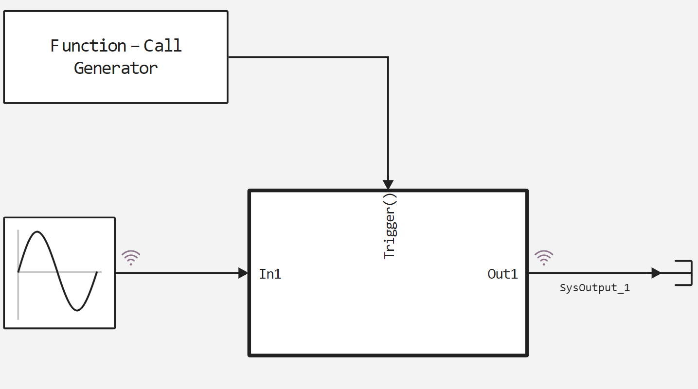
The subsystem for calling functions is similar to a function in a procedural programming language. Calling the function call subsystem triggers the block output methods within the subsystem in the order of execution. The figures below show an example of using a Function-Call Generator and Function-Call Subsystems.
.png)
.png)
run_model("function_call",path) # Launching the model.
# Reading of encoded signals from simout
out = simout["function_call/SysOutput_1"];
out = collect(out);
inp = simout["function_call/Sine Wave.1"];
inp = collect(inp);
The input sinusoid.
plot(inp.time,inp.value)
The output amount.
plot(out.time,out.value)
As we can see in this example, according to the condition of the control function, the counter increment is performed inside the subsystem.
Conclusion
In this demo, we have analyzed all the Subsystems options that you can find in Engee and use in your projects.