Bouncing ball simulation
This example shows how to perform a bouncing ball simulation in Engee.
First, we will declare a function to run the model and the library that we will need when working with data from the model.
 using Plots

 function run_model(name_model)
    Path = (@__DIR__) * "/" * name_model * ".engee"

    if name_model in [m.name for m in engee.get_all_models()] # Checking the condition for loading a model into the kernel
        model = engee.open( name_model ) # Open the model
        model_output = engee.run( model, verbose=true ); # Launch the model
    else
        model = engee.load( Path, force=true ) # Upload a model
        model_output = engee.run( model, verbose=true ); # Launch the model
        engee.close( name_model, force=true ); # Close the model
    end

    return model_output
end
Let's move on to the theoretical component of this demonstration. The figure below shows the basic principle behind the demonstration. Conditions: the ball was thrown at a speed of 15 m/s from a height of 10 m.
The bouncing ball model is a classic example of a hybrid dynamic system. A hybrid dynamic system is a system that includes continuous dynamics as well as discrete transitions where system dynamics can change and state values can transition.
The continuous dynamics of a bouncing ball is described in a simple way as follows:
.png)

where: acceleration is due to gravity, – the position of the ball and – speed. Therefore, the system has two continuous states: position and the speed .
The aspect of the hybrid model system comes from simulating the collision of a ball with the ground. If you assume a partially elastic impact with the ground, then the velocity before the collision is and the speed after the collision may be related to the recovery rate of the ball as follows:
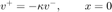
A bouncing ball therefore displays a jump in a continuous state (velocity) under the condition of transition .
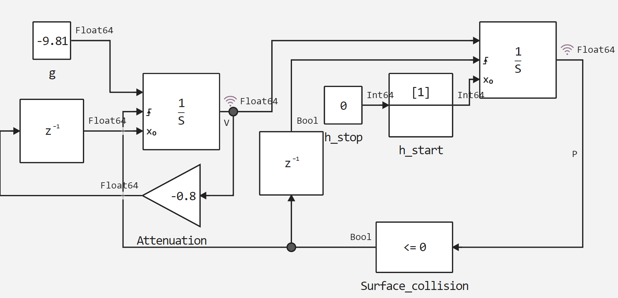
Let's move on to launching the model and analyzing the data. The model itself is shown in the picture below.
.png)
h_start = 10; # Height
v_start = 15; # Speed
run_model("bouncing_ball")
sleep(5)
collect(simout)
Let's build graphs based on the aggregated data, and also, for visual convenience, we'll build a graph with the zero Y axis.
# Speed
v = simout["bouncing_ball/V"];
v = collect(v);
plot(v.time, v.value, label="Speed")

# Position
p = simout["bouncing_ball/P"];
p = collect(p);
plot!(p.time, p.value, label="Position")

plot!(p.time, zeros(size(p.time)))
Conclusion
In this example, we have built a simulation of a bouncing ball, and also considered the possibilities of interacting with the simulation environment from Engee scripts.
Bouncing ball is one of the simplest models that shows the phenomenon of Zen. Zen behavior is informally characterized by an infinite number of events occurring over a finite period of time for certain hybrid systems. When the ball loses energy in the bouncing ball model, a large number of collisions with the ground begin to occur in successively shorter time intervals. Hence, the model experiences Zen behavior. Zen behavior models are not easy to simulate on a computer, but they are necessary because they are found in many common and important engineering applications.