Van der Polye oscillator

This example shows how to model a second order Van der Polye differential equation (VDP) in Engee. In dynamics, the oscillator is non-conservative and has nonlinear damping. At large amplitudes, the oscillator dissipates energy. At small amplitudes, the generator generates energy.

The oscillator is given by a second order differential equation:

Where:

1. x is the position relative to time.
2. t - time
3. Mu - attenuation.

The VDP generator is used in biological and physical sciences, including electrical circuits.

Next, let's move on to implementation - declare the function to run the model and connect the necessary libraries.

 using Plots

 function run_model(name_model)
    Path = (@__DIR__) * "/" * name_model * ".engee"

    if name_model in [m.name for m in engee.get_all_models()] # Проверка условия загрузки модели в ядро
        model = engee.open( name_model ) # Открыть модель
        model_output = engee.run( model, verbose=true ); # Запустить модель
    else
        model = engee.load( Path, force=true ) # Загрузить модель
        model_output = engee.run( model, verbose=true ); # Запустить модель
        engee.close( name_model, force=true ); # Закрыть модель
    end

    return model_output
end

run_model (generic function with 1 method)

Let's run the model with several variants of Mu value. Further in the figure you can see the model we made based on the formula described above.

The attenuation coefficient is equal to one

Set Mu and run the model, then analyse the logged data.

Mu = 1;
run_model("vdp")
sleep(5)
collect(simout)

Building...
Progress 100%

2-element Vector{WorkspaceArray}:
 WorkspaceArray("vdp/Integrator.1")
 WorkspaceArray("vdp/Integrator-1.1")

# Скорость
v = simout["vdp/Integrator.1"];
v = collect(v);
plot(v.time, v.value)

# Положение
p = simout["vdp/Integrator-1.1"];
p = collect(p);
plot!(p.time, p.value) 

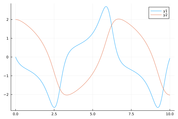
As we can see from the resulting graph, at Mu = 1 the VDP generator has non-linear damping.

The attenuation coefficient is equal to zero

Set Mu and run the model, then analyse the logged data.

Mu = 0;
run_model("vdp")
sleep(5)
collect(simout)

Building...
Progress 100%

2-element Vector{WorkspaceArray}:
 WorkspaceArray("vdp/Integrator.1")
 WorkspaceArray("vdp/Integrator-1.1")

# Скорость
v = simout["vdp/Integrator.1"];
v = collect(v);
plot(v.time, v.value)

# Положение
p = simout["vdp/Integrator-1.1"];
p = collect(p);
plot!(p.time, p.value) 

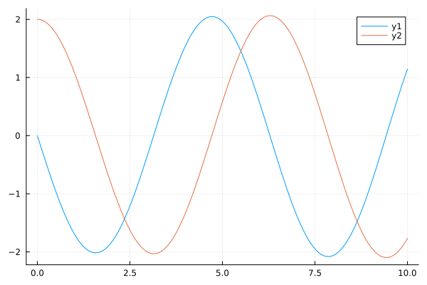
Analysing the graph, we can conclude that at Mu = 0 the VDP generator has no damping, the energy is conserved, and the differential equation itself takes the following form:

Conclusion

In this example, we have modelled the second order van der Pol differential equation in Engee and seen how it performs with different values of the damping factor.

Blocks used in example

• Gain
• Integrator
• Divide
• Add