Creating Engee Function blocks with state variables¶

In this example, we will create a block Engee Function, whose parameters can change over time depending on various factors. Usually the output of a custom block is calculated based on the input data and the time vector. But in this example we will show how to work with variables that can store the internal state of the block.

In practical terms - we will show how to change the result of the custom block calculation depending on the internal execution counter implemented inside the block.

Organisation of Engee Function block parameters¶

The parameters of the block Engee Function can be set in different ways:

by means of constants, through the settings window Parameters
using variables from the global variable space Engee (visible in the Variables window)
with the help of internal parameters of the block, specified in its code (and the time of their existence is not limited by the next cycle of calculations, but is equal to the time of model existence).

The first two variants are realised almost identically. If the number of parameters is non-zero, then for each of them it is necessary to set the name Name and the value Value.

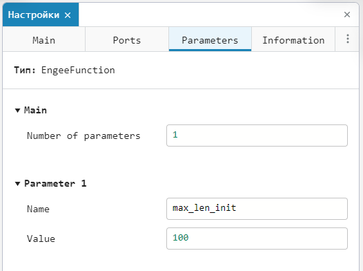
Here we have set the size of the window for calculating statistical parameters max_len_init and assigned the value 100.

We could have assigned to it the value N, set in the global variable space. We should keep in mind a limitation of the model compiler: when passing a variable from the global space, the name of the parameter (Name) must not be identical to the name of the global variable (Value).

This temporary compiler behaviour will be fixed soon.

Variable parameters in Engee Function code¶

Let's consider a practical example. We are going to implement a block that calculates statistical parameters of the part of the sample that falls into a sliding window of a given size. The window will be initialised with a zero value, so the first N results will be biased, but then we will see the statistics for the sliding window including the last N values from the observed sample.

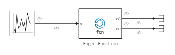
The Engee Function block will take scalar values as input and accumulate statistics on them. The block of noise generation - a uniformly distributed random variable with values in the interval (-1,1) - will be at the input. The interface of the block will look as follows:

Here MA stands for Moving Average (moving average) and MD stands for Moving Deviation (moving variance).

It is worth commenting each section of the code that defines the behaviour of our custom block.

The code starts with initialisation of the user block structure. The name Block is chosen randomly, it can be anything. Inside we set several parameters:

i - counter of the last added element in the cyclic accumulator
max_len - size of the sliding window
X - sampling accumulator (vector of max_len size)

In the Block() function, internal parameters receive specific values, including those received from outside (the size of the max_len_init window is set on the Parameters tab ).

Parsing the code inside the Engee Function component¶

We should be careful about assigning data types to block parameters. If you don't declare the data structure defining the state variables as a structure of type mutable, then all "simple" types within the structure will be unchanged (you will have to use vectors or references, e.g. i :: Ref{Int32};). We want to be able to modify the parameters. Therefore, we set a special modifier to our structure:

mutable struct Block <: AbstractCausalComponent

    i :: Int32;
    max_len :: Int32;
    X :: Vector{Float64};

    function Block()
        return new( 1, max_len_init, zeros(Float64, max_len_init) ) )
    end

end

Then in the code we see a function that is evaluated each time the block is accessed.

It is very important that when this function is called, its internal variables are not changed. The method (functor) step can be called many times between simulation steps, so if you change the internal state of the block in it, it will change too often.

Here we can refer to external and internal parameters of the block (c.параметр).

function (c::Block)(t::Real, x)

    # Local variables are for readability only
    X = c.X
    N = c.max_len

    MA = sum( X[1:N] )/N;
    MD = sqrt( sum( (X[1:N] .- MA).^2 ) / (N-1) )

    return (MA, MD)
end

Finally we see the function update!, which is designed to make changes to the parameters of the block c.

We substitute the current value of x with the block input Engee Function into the vector X at index i;
Then we increase by 1 the index i, and when it reaches the value max_len, we decrease it back to one;
Finally, we return the updated parameter structure c to refer to it at the next iteration.

function update!(c::Block, t::Real, x)
    
    c.X[c.i] = x
    c.i = max(1, (c.i + 1) % (c.max_len-1))
    
    return c
end

The code inside update! is especially important when the Engee Function block is in an algebraic loop (e.g., it takes its own outputs as input, or has an exposed parameter direct_feedthrough=false). In models where there is no loop, everything can be done in the second code block (functor step).

Running the model and discussing the results¶

Let's run this model using program control commands:

mName = "engee_function_moving_average"
model = mName in [m.name for m in engee.get_all_models()] ? engee.open( mName ) : engee.load( "$(@__DIR__)/$(mName).engee" );
data = engee.run( mName )

Dict{String, DataFrame} with 3 entries:
  "MA"  => 501×2 DataFrame…
  "src" => 501×2 DataFrame…
  "MD"  => 501×2 DataFrame…

Output the result:

using Plots, Formatting

p = plot( data["MD"].value, data["MA"].value, label="MA(MD)", linez=range(0.4, 1, length(data["MA"].value)), c=:blues, cbar=:none)
# Последняя точка на графике
scatter!( p, [data["MD"].value[end]], [data["MA"].value[end]], c=:cyan )
# Текстовая подпись к этой точке 
annotate!( p, data["MD"].value[end], data["MA"].value[end],
           text("MA=$(sprintf1("%.2f",data["MD"].value[end])), MD=$(sprintf1("%.2f",data["MA"].value[end]))  ", 8, :right ),
           legend=:none )

# Вывод двух графиков
plot(
    # График слева: шум
    plot( data["src"].time, data["src"].value, label="input", c=:red, legend=:none ),
    # График справа – зависимость мат.ожидания от дисперсии
    p,
    size=(800,300)
)

The left graph shows the noise signal that was input to the user block Engee Function. The right graph shows the dependence of the moving average on the variance value for the sliding window.

It can be noted that the starting point of the mean and variance was the value for the zero sample, but after several tens of steps the estimation of these parameters shifted to the point $\mu \approx -0.15$, $\sigma \approx 0.55$. By the end of the calculation period, when the initialisation of the sliding window stopped affecting the statistics, the point on the graph began to shift noticeably to the zero mathematical expectation at $\sigma \approx 0.6$.

Conclusion¶

If you add a few standard constructs to the original code pattern in a Engee Function component, you can embody very complex behaviour in that component, relying on external code and changeable parameters. In Engee there are many graphical and textual ways to describe the behaviour of models, in addition to which you can use dynamic blocks with custom code inside.