Comparison of subsystems included
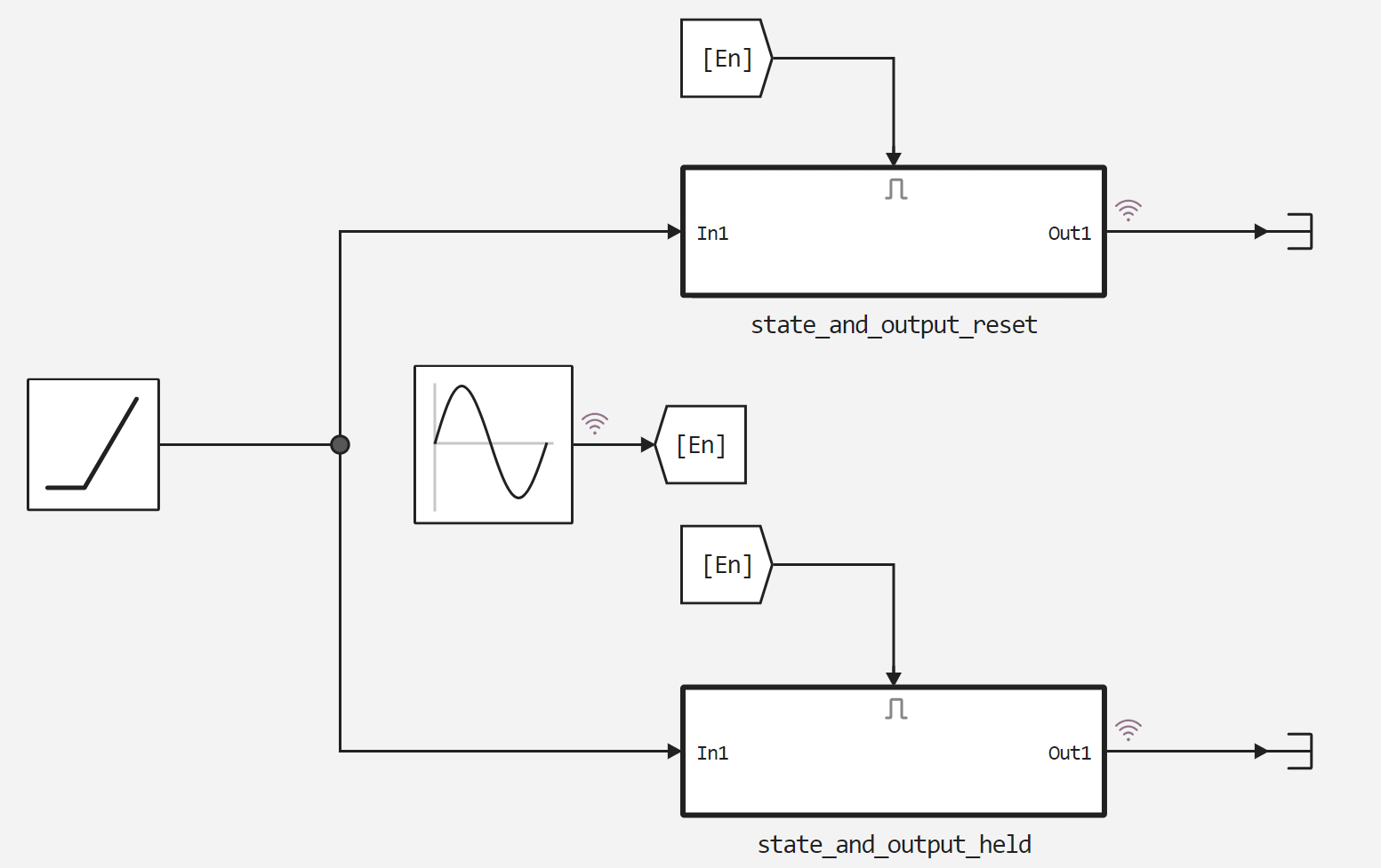
In this example, a variant of two identical subsystems is analyzed, with differences in the settings of the received control signal. In the first case, the signal starts the model, in the second it resets its execution.
The picture below shows the model itself.
Next, we'll connect an auxiliary function to launch the model.
In [ ]:
function run_model( name_model)

    Path = (@__DIR__) * "/" * name_model * ".engee"

    if name_model in [m.name for m in engee.get_all_models()] # Checking the condition for loading a model into the kernel
        model = engee.open( name_model ) # Open the model
        model_output = engee.run( model, verbose=true ); # Launch the model
    else
        model = engee.load( Path, force=true ) # Upload a model
        model_output = engee.run( model, verbose=true ); # Launch the model
        engee.close( name_model, force=true ); # Close the model
    end
    sleep(5)
    return model_output
end
Out[0]:
Let's launch the model.
In [ ]:
run_model("CompareEnabled") # Launching the model.
Out[0]:
Let's unpack and display the signals recorded from the model.
In [ ]:
held = simout["CompareEnabled/state_and_output_held.Out1"];
reset = simout["CompareEnabled/state_and_output_reset.Out1"];
Sine = simout["CompareEnabled/Sine Wave.1"];

held = collect(held);
reset = collect(reset);
Sine = collect(Sine);

plot(held.time, held.value)
plot!(reset.time, reset.value)
plot!(Sine.time, Sine.value)
Out[0]:
Conclusion
As we can see from the resulting graph, the reset system switches to the initial state of the integrator at the moment of transition to the positive region of the control signal, while the system continues counting from the last calculated value inside the integrator without reset.