Mathematical models of bodies
In this example, we will consider two body models. In the first case, it will be a pendulum, and in the second, a body on a spring. Let's analyze the behavior of these bodies.
The mathematical pendulum
Let's look at the process of describing oscillatory systems using integral calculations in the Engee development environment. The figure shows a model of an oscillatory system.:
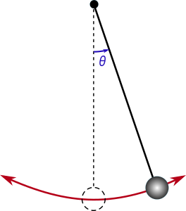
The model includes several basic concepts:
- The material point of mass is m.
- Weightless inextensible thread length l.
- Homogeneous gravitational force field g.
In this case, the formula for calculating the moment of gravity is is equal to the negative value of the mass multiplied by and and the sine of the angle of deflection of the pendulum.
Let's move on to implementation. The first step is to announce the system parameters.
Pkg.add(["CSV"])
m = 1;
g = 9.8;
l = 1;

theta_init = 40*(pi/180); # converting the initial value of the degree of deviation to radians

mgl=(-m*g*l);
invI = 1/(m * l^2);
Now let's run the system of integral equations built in the Engee models. The picture below shows this model:
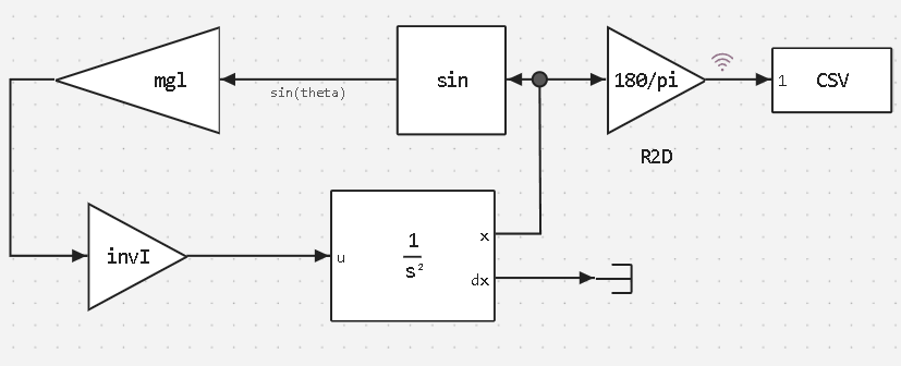
Note: The solver AB3 was used in the simulation.
_AB3 is a third–order three-step method, initialization of second-order Ralston methods.
# Launching the model
model = engee.load("/user/start/examples/base_simulation/mathematical_models_of_bodies/Math_pendulum.engee"; force = true);
engee.run(model, verbose=true);
engee.close(model, force=true);
To process and visualize the simulation results, we need to connect several libraries.
using CSV
using DataFrames
using Plots
plotlyjs()
Now we can read the data recorded during the simulation. The data in the CSV file contains two columns:
- timestamps of the simulation;
- Output data, in this case the values of the degree of deviation of the pendulum.
# Reading CSV
Data = Matrix(CSV.read("/user/start/examples/base_simulation/mathematical_models_of_bodies/out.csv",DataFrame));
Data_time = Data[:,1];
Data = Data[:,2];
Now let's analyze the results of the oscillation, presenting them graphically.
# Plotting graphs
plot(Data_time , Data, legend = false)
plot!(title = "Simulation results in Engee", ylabel = "Data", xlabel="Time, c")
As we can see, the model displays non-decaying oscillations of a mathematical pendulum with a constant oscillatory process.
Mathematical model of mass-spring-damper
In this example, we will demonstrate the possibilities of calculating the behavior of a body on a spring in order to demonstrate the capabilities of Engee in solving integral equations. The figure below shows the general view of the body for which calculations will be performed.
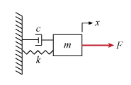
The mass spring damper shown in the figure is modeled by a second-order differential equation.
where is the force applied to the mass, and – horizontal position of the mass.
Let's move on to implementation. First, we will announce the system parameters.
m = 2;
c = 50;
k = 0.2;

invM = 1/m;
Now let's run the system of integral equations built in the Engee models. The picture below shows this model:
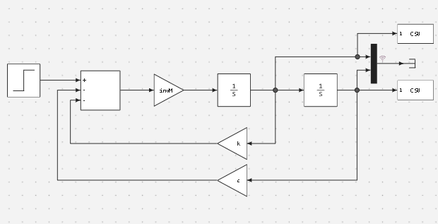
Note: The solver AB3 was used in the simulation.
_AB3 is a third–order three-step method, initialization of second-order Ralston methods.
# Launching the model
model = engee.load("/user/start/examples/base_simulation/mathematical_models_of_bodies/Body_on_spring.engee", force=true);
engee.run(model, verbose=true);
engee.close(model, force=true);
To process and visualize the simulation results, we need to connect several libraries.
using CSV
using DataFrames
using Plots
plotlyjs()
Now we can read the data recorded during the simulation. The data in the CSV file contains two columns:
- timestamps of the simulation;
- Output data.
# Reading CSV
Data1 = Matrix(CSV.read("/user/start/examples/base_simulation/mathematical_models_of_bodies/out1.csv",DataFrame));
Data2 = Matrix(CSV.read("/user/start/examples/base_simulation/mathematical_models_of_bodies/out2.csv",DataFrame));

Data_time = Data1[:,1];
Data1 = Data1[:,2];
Data2 = Data2[:,2];
Now let's analyze the results of the oscillation and present them graphically.
# Plotting graphs
plot(Data_time , Data1, legend = false)
plot!(Data_time , Data2, legend = false)
plot!(title = "Simulation results in Engee", ylabel = "Data", xlabel="Time, c")
As we can see, the model displays vibrations with a gradual attenuation of the oscillatory process, which is identical to the behavior of a physical body on a spring.
Conclusion
As a result of the implementation of this example, we have shown you the capabilities of Engee in modeling the behavior of physical objects by constructing a mathematical model of the object.
This example allows you to demonstrate the behavior of an object based on its parameters, which can be applicable to more complex algorithms and systems.