Calculating the approximate value of a function
In this demonstration, we will look at the possibilities of calculating approximate values of a function using Engee and examine the basic blocks used to solve this problem.
Block Analysis
The Prelookup block calculates the number and fraction of the interval, which determine how its input value u relates to a set of reference points.
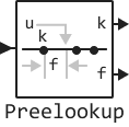
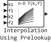
The Interpolation Using Prelookup block is most effective when using the Prelookup block. The Prelookup block calculates the index and fraction of the interval, which determine how its input value u relates to the data set of breakpoints. The resulting index and fraction values are fed into the Interpolation Using Prelookup block for interpolation of an n-dimensional table. Both blocks have integrated algorithms.
The n-D Lookup Table block calculates the approximate value of a function. This block and its variants compare input data with a table of output values using interpolation and extrapolation methods.
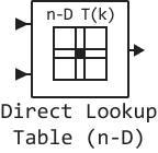
The Direct Lookup Table (n-D) block indexes an n-dimensional table to extract a scalar, vector, or two-dimensional matrix. The first selection index corresponds to the upper (or left) input port. You can specify the table data as input to the block, or define the table data in the block dialog box. The number of input ports and the size of the output depend on the number of table sizes and the selected output slice.
Model implementation
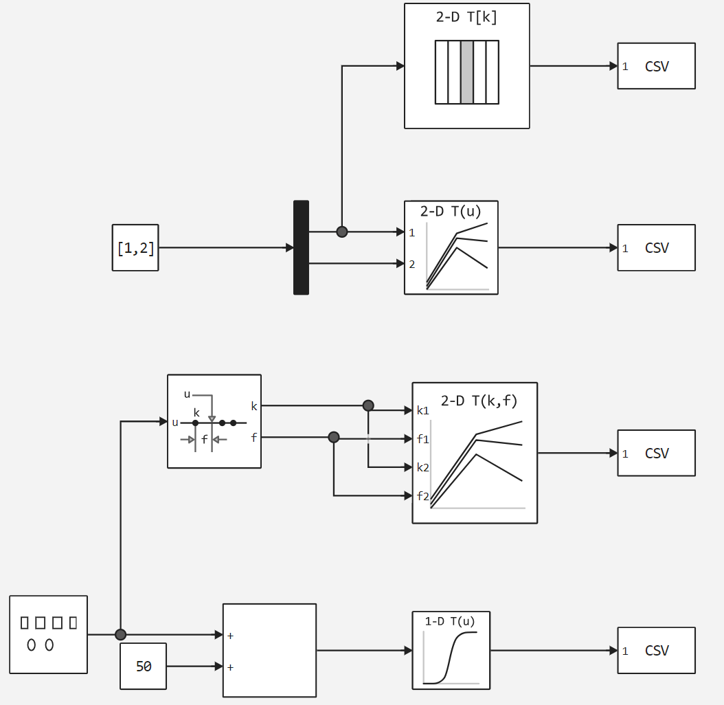
Next, let's look at the model using all the blocks listed above.
.png)
Now let's add initialization of tables and search points for the model. Let's start with the Direct Lookup Table (n-D) and 2-D Lookup Table blocks, and connect the libraries necessary for data processing and visualization.
# Connecting libraries
using DataFrames
using Plots
Points2D = [1, 2, 3]; # Indexing points
Matrix2D = [4 50 6; 16 19 20; 10 18 23] # Table
# Reading points
X = 1;
Y = 2;
idx = [X,Y];
# Reading points
X = 1;
Y = 2;
idx = [X,Y];
Now let's initialize Prelookup and Interpolation Using Prelookup, and also plot the ratio of points to the table.
Value1 = 10:10:110; # Points
Value2 = sqrt.(collect(1:11) * collect(1:11)'); # Таблица
plot(Value1, Value2)
The last block with no initialization parameters declared is the 1-D Lookup Table.
Points1D = 1:1:100; # Indexing points
Matrix1D = sin.(1:2:200); # Table
A = 50; # The amplitude of the signal generator
plot(Points1D,Matrix1D)
Let's run the model with the specified parameters.
function run_model( name_model, path_to_folder )

    Path = path_to_folder * "/" * name_model * ".engee"

    if name_model in [m.name for m in engee.get_all_models()] # Checking the condition for loading a model into the kernel
        model = engee.open( name_model ) # Open the model
        model_output = engee.run( model, verbose=true ); # Launch the model
    else
        model = engee.load( Path, force=true ) # Upload a model
        model_output = engee.run( model, verbose=true ); # Launch the model
        engee.close( name_model, force=true ); # Close the model
    end

    return model_output
end
res = run_model("Lookup_Table","/user/start/examples/base_simulation/lookup_table")
Let's consider the simulation results contained in the res variable.
In the first case, we counted a column from Matrix2D.
df = collect(res["Direct Lookup Table (n-D).1"]);
println(df[1,2])
In the second case, we counted the values from Matrix2D into cells [X,Y].
df = collect(res["2-D Lookup Table.1"])
println(df[1,2])
In the third case from Interpolation Using Prelookup we are reading from the data from Prelookup.
df = collect(res["Interpolation Using Prelookup.1"])
plot(df[!,2])
And in the latter case, we read the sinusoid from the 1-D Lookup Table.
df = collect(res["1-D Lookup Table (mod.).1"])
plot(df[!,2])
Conclusion
As a result of this demonstration, we have shown how to use various blocks for calculating the approximate value of a function.
We also implemented two functions:
- launching the model;
- Parsing the CSV with the matrix written in it.