Conclusion of graphs in the polar coordinate system
In this example, we will show how to display a graph in the polar coordinate system for the dynamic Engee model.
Polar graph in an interactive script
Graphs in a polar coordinate system allow you to see relationships that are not visible on graphs in a rectangular (Cartesian) coordinate system: to get an idea of the severity of a certain process in certain directions in space, or to track repetitive dynamics within a cyclical process...
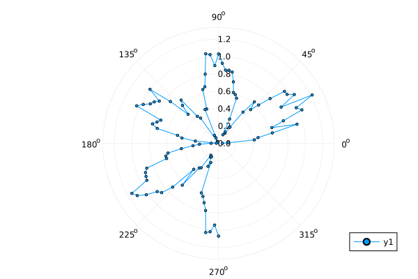
If the work is carried out in an interactive script Engee, then the graph is translated to the polar coordinate system using the argument proj. Its value :polar allows us to plot a graph in polar coordinates:
Θ = range( 0, stop = 1.5π, length = 100 )
r = abs.( 0.1 * randn(100) + sin.(3Θ) )
plot( Θ, r, proj = :polar, m = 2 )
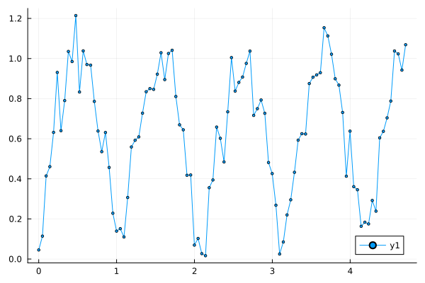
While the parameter ortho plots a graph in a rectangular coordinate system
plot( Θ, r, proj = :ortho, m = 2 )
Let's try to graph in the polar coordinate system, using only the canvas and tool output graphs for dynamic models ().
Polar graph for a dynamic model
To build a polar graph for a dynamic model without using interactive script tools, we will need to convert vectors from a rectangular coordinate system to a polar system.
Consider the following model (draw_polar_engee_logo.engee):
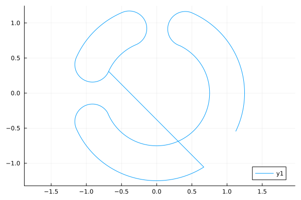
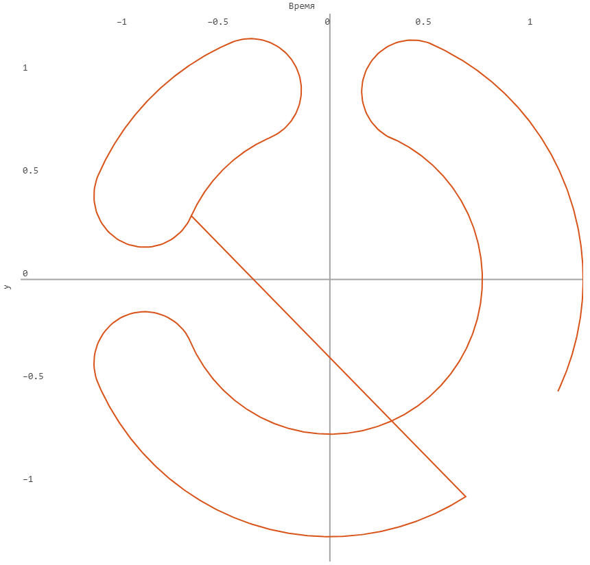
If you run it using the , it will plot the following graph:
Let's analyze this model using [software modeling management] tools (https://engee.com/helpcenter/stable/modeling/programmatic-modeling-editing.html ).
modelName = "draw_polar_engee_logo";
model = modelName in [m.name for m in engee.get_all_models()] ? engee.open( modelName ) : engee.load( "$(@__DIR__)/$(modelName).engee");
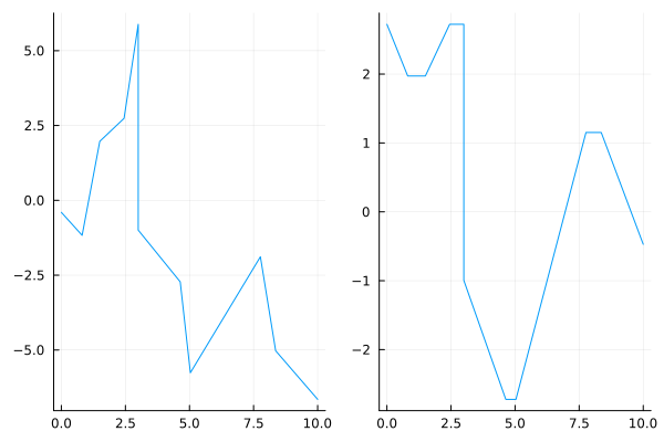
We can study which piecewise linear dependencies are given in each block. LUT without running the simulation, but simply by accessing the properties of each block.
# Analyzing the first table of substitutions
x1 = eval(Meta.parse(engee.get_param( modelName*"/LUT1", "BreakpointsForDimension1" )));
y1 = eval(Meta.parse(engee.get_param( modelName*"/LUT1", "Table" )));

# Let's analyze the second table of substitutions
x2 = eval(Meta.parse(engee.get_param( modelName*"/LUT2", "BreakpointsForDimension1" )));
y2 = eval(Meta.parse(engee.get_param( modelName*"/LUT2", "Table" )));

# Let's build a graph
plot(
    plot( x1, y1, legend=false ),
    plot( x2, y2, legend=false )
)
As a result, the model builds a graph in a rectangular coordinate system, but outputs them after a transformation that interprets the input signals as data in a polar coordinate system.
The output graph is the sum of two graphs in the polar coordinate system. The first one sets the position of the center line of each of the two curves that make up the logo (curve LUT2, its radius 1.0). The second component (curve LUT1, output with a radius of 0.25) simulates the deviation from the center line.
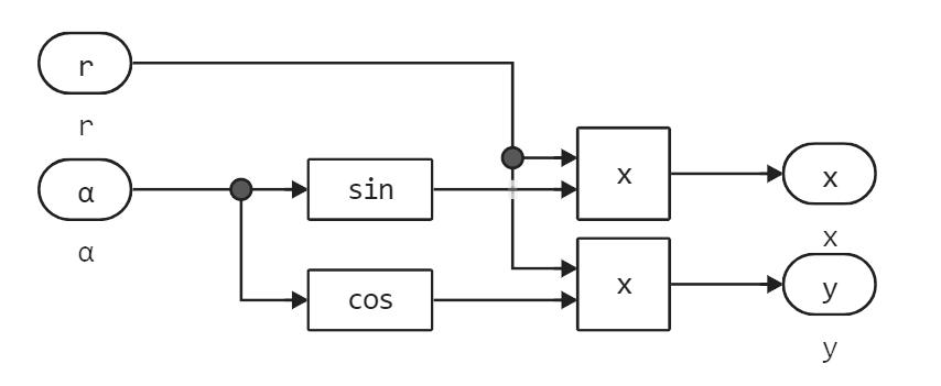
The coordinate transformation is done in two different ways. Both options are interchangeable. In the first case, we will transform the coordinates using simple blocks from the basic palette.:
.png)
In the second case, we use the block Engee Function with the following code performing the same operations:
struct Block <: AbstractCausalComponent
    # Нет параметров
end

function (c::Block)(t::Real, α, r)
    x = r * sin( α )
    y = r * cos( α )
    return (x,y)
end
Let's output the graph that our model builds.:
gr()
s = engee.run( modelName, verbose=false );
plot( s["y"].value, s["x"].value, aspect_ratio=:equal )
Conclusion
Engee is gradually introducing more and more sophisticated charting tools that you can work with without resorting to programming.
In this demo, we showed how to plot a graph in polar coordinates without resorting to programming and how to do it using the block Engee Function.
Unlike the graphs in an interactive script, the graphs of dynamic models can be updated directly during the simulation, which creates interesting opportunities for interactive simulation of models.
