Using the Variant Source and Variant Sink blocks
In this example, we will show how the blocks work. Variant Source and Variant Sink. These blocks allow you to switch between different model implementations, which are generators of input data or consumers of output data of some subsystem.
Introduction
Suppose you need to calculate the operation of a model with different input sensors, different cyclograms, or different algorithms for filtering data at the output. For such testing, you can assemble several separate models, the number of which will quickly become impractically large. Or you can assemble all the models into one and switch the conditions using variables.
In this simplified example, the model configuration will be set by two scalar variables.:
Pkg.add(["Combinatorics"])
V = 1;
W = 1;
The model has several signal line switches controlled by external variables.
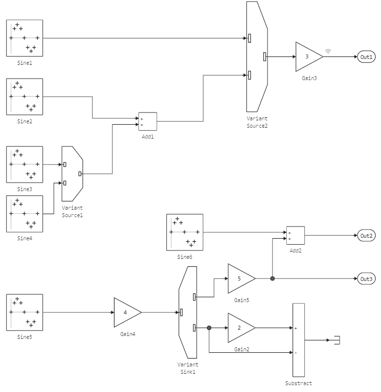
Signal selection conditions in each block Variant Source or Variant Sink they are set using expressions.
The expression that first takes the true value defines the port number through which the data will go from or to some subsystem. Let's interpret the different variants of the systems that are implemented in this scheme.:
- If
W==1is the true expression of theVariant Source1activates the inputSine3, and whenV==4the entrance is activatedSine4. - When
V==1blockVariant Source 2skips the signal from the blockSine1, and whenV==2– signal from the unitAdd1. - If the block
Add1inactive, thenVariant Source 1It will also be inactive, and then the blocks will be disabled.Sine3andSine4(blockSine3active whenV==2 && W==1, and the blockSine4active whenV==2 && W==2). - Yulok
Gain3active either whenV==1, or whenV==2; under other conditions (for example , whenV=4) we will get an error because on the output portOut1no output signal will be given. - Blocks at the exit
Variant Sink1they become active whenW==1 (Gain5)or whenW==2 (Gain2, Substract, Terminator). - Finally, the blocks
Sine6,SumandOut2they are always active, they are not subject to the conditions for choosing system options. To ensure that these blocks are executed only under certain conditions, you can put blocks before and after them.Variant Source/Sinkboth with a single entrance and exit.
Under some combinations of conditions, this model returns an error because the subsystem's output ports must receive an active signal regardless of the subsystem's variant. It is not possible to send an active and inactive signal to any block at the same time, it is necessary to explicitly design the output ports of such a system using blocks Variant Source/Sink to set default values.
Running the script
mName = "variant_source_sink"
model = mName in [m.name for m in engee.get_all_models()] ? engee.open( mName ) : engee.load( "$(@__DIR__)/$(mName).engee" );
data = engee.run( mName )
plot( data["Gain3.1"].time, data["Gain3.1"].value )
Running multiple scripts
Now we will run several variants of the model in a loop, switching state variables in order to use a combination of input conditions to show how the system works in different scenarios.
using Combinatorics
# We will set all the input conditions we are interested in
vV = [1,2,4];
vW = [1,2,4];

# Loading the model
mName = "variant_source_sink"
model = mName in [m.name for m in engee.get_all_models()] ? engee.open( mName ) : engee.load( "$(@__DIR__)/$(mName).engee" );

# We will store the success of the execution in a matrix, which we initialize with the missing values.
run_success = NaN .* zeros(length(vV), length(vW))

# Let's go through all the combinations of input conditions and check if the model holds.
for c in combinations( vcat( vV,vW ), 2  )
    V,W = c[1],c[2]
    i = findfirst( vV.==c[1] )
    j = findfirst( vW.==c[2] )

    try
        # Let's run the model for execution
        data = engee.run( mName )
    catch e
        # If the model was executed with an error, write 0 to the output matrix.
        run_success[i,j] = 0
    else
        # We'll write one only if the catch condition didn't work.
        run_success[i,j] = 1
    end

end
Let's display a graph on which statistics on launches of different variants of our model will be collected.
gr()
# Output of a non-interactive map reflecting the success of the model
heatmap( run_success, xticks=(range(1,length(vV)), vV), yticks=(range(1,length(vW)), vW),
         xlabel = 'V', ylabel='W', title="Model execution success", yflip = true, cbar=false, c=:Blues )
# Annotation on top of each cell
annotate!( vec(tuple.((1:length(vV))', (1:length(vW)), string.(Int32.(run_success)))) )
Conclusion
We have seen that several system variants can be assembled on one canvas. This method simplifies testing and allows you to generate many code variants at once to further automate semi-natural modeling.