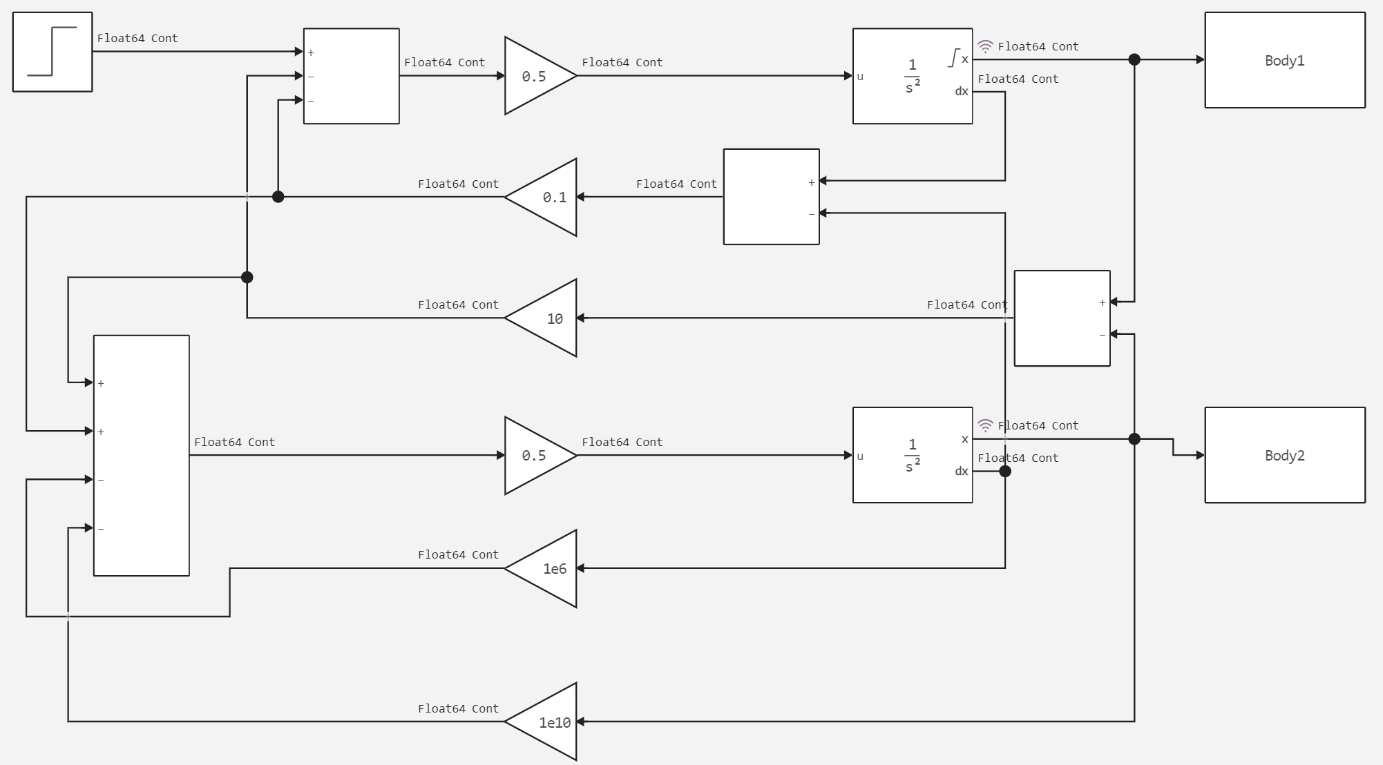
Rigid mechanical system
You've seen how the solver settings can affect the simulation process – its speed and outcome.
This example presents a model of a rigid mechanical system using a variable-pitch solver.
This rigid system includes two oscillating masses, each with a different calculation step. The picture below shows the system itself.
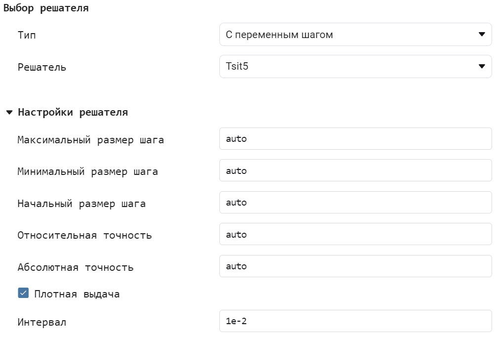
The following shows the solver settings.
Now let's move on to running the model and analyzing the results. To do this, we will need to declare an auxiliary function.
In [ ]:
# Enabling the auxiliary model launch function.
function run_model( name_model)

    Path = (@__DIR__) * "/" * name_model * ".engee"

    if name_model in [m.name for m in engee.get_all_models()] # Checking the condition for loading a model into the kernel
        model = engee.open( name_model ) # Open the model
        model_output = engee.run( model, verbose=true ); # Launch the model
    else
        model = engee.load( Path, force=true ) # Upload a model
        model_output = engee.run( model, verbose=true ); # Launch the model
        engee.close( name_model, force=true ); # Close the model
    end
    sleep(5)
    return model_output
end

run_model("stiffMechanicalSystem") # Launching the model.
Out[0]:
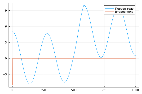
Let's build the resulting graph.
In [ ]:
Body1 = collect(Body1);
Body2 = collect(Body2);
In [ ]:
gr()
plot(Body1.value, label = "The first body")
plot!(Body2.value, label = "The second body")
Out[0]:
Conclusion
As we can see on the graph, the second body is at rest, while the first body makes oscillatory movements.