Integrating Julia code into Engee models using the Engee Function block
This example shows a way to integrate Julia code into the Engee model using the Engee Function block.
Before starting work, we will connect the necessary libraries.:
Pkg.add(["Statistics", "ControlSystems", "CSV"])
using Plots
using MATLAB
using CSV
using Statistics
using ControlSystems
plotlyjs();
Using a macro @__DIR__ in order to find out the folder where the interactive script is located:
demoroot = @__DIR__
Setting the task
Let's assume that we are interested in filtering noisy angular position measurements. a pendulum using a Kalman filter.
Let's determine the gain of the Kalman filter using the library [ControlSystems.jl](https://juliacontrol.github.io/ControlSystems.jl/stable /) and integrate the Julia code implementing the filter into the Engee model using the Engee Function block.
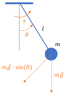
Simplified mathematical model of a pendulum in the state space
To implement the Kalman filter, we need a model of a pendulum in the state space.
A simple frictionless pendulum system can be represented by the equation:
This equation can be rewritten as follows:
For small angles :
Replace the torque to the input vector and let's represent the linearized system as a model in the state space.:
Then the state space matrices will be defined as follows:
Signal filtering in Engee using the Engee Function block
Model analysis
Let's analyze the model juliaCodeIntegration.engee.
The upper level of the model:
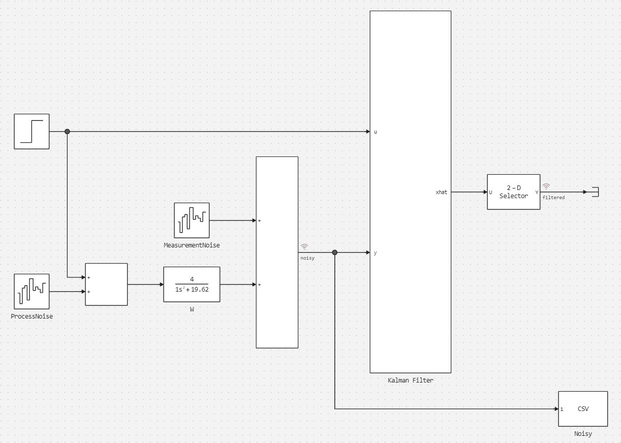
The pendulum is represented by a transfer function:
In Blocks Band-Limited White Noise ProcessNoise and MeasurementNoise The external impact and measurement noise are presented.
Subsystem Kalman Filter:
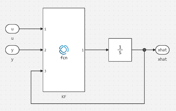
Block Settings KF (Engee Function):
- Tab
Main:
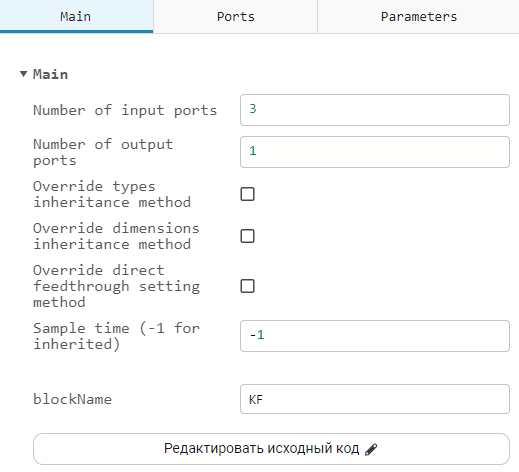
The number of input and output ports is determined by the properties Number of input ports and Number of output ports.
- Tab
Ports:
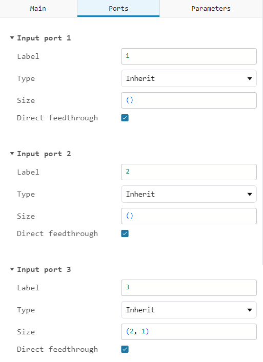
The dimension of the input and output signals is determined by the Size property:
- Two scalar signals and a vector are applied to the input of the unit.
[2x1]; - one vector is formed at the output
[2x1].
- Tab
Parameters:
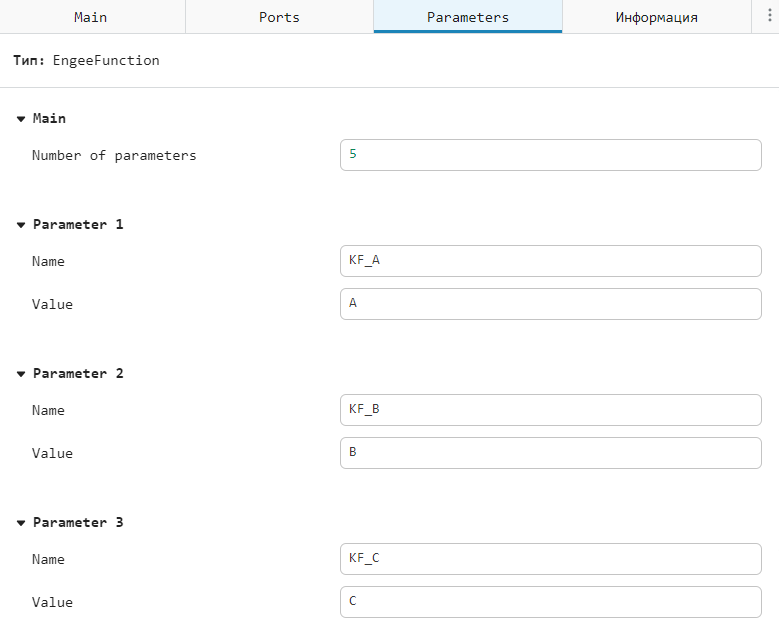
Parameters KF_A, KF_B, KF_C, KF_D, KF_K variables are compared A, B, C, D and K from the Engee workspace. Their values will be defined in the section "Starting the simulation".
Contents of the ExeCode block tab KF:
include("/user/start/examples/base_simulation/juliacodeintegration/filter.jl")

struct KF <: AbstractCausalComponent; end

function (kalman_filter::KF)(t::Real, u, y, x)
    xhat = xhat_predict(u, x, KF_A, KF_B) + xhat_update(u, y, x, KF_C, KF_D, KF_K)

    return xhat
end
Structure KF inherited from AbstractCausalComponent.
Line include("/user/start/examples/base_simulation/juliacodeintegration/filter.jl") required to connect an external source code file filter.jl.
In the file filter.jl The functions are defined xhat_predict and xhat_update designed to generate an output signal xhat the block KF:
function xhat_predict(u, x, A, B)
    return (B * u) + (A * x)
end

function xhat_update(u, y, x, C, D, K)
    return (K * (y .- ((C * x) .+ (D * u))))
end
In this example, there are no internal states, so the method update!, designed to update them, is missing.
Running the simulation
Loading the model juliaCodeIntegration.engee:
juliaCodeIntegration = engee.load("$demoroot/juliaCodeIntegration.engee", force = true)
And initialize the variables necessary to simulate it.:
g = 9.81;
m = 1;
L = 0.5;

Ts = 0.001;
Q = 1e-3;
R = 1e-4;

processNoisePower = Q * Ts;
measurementNoisePower = R * Ts;
Let's form a model of a pendulum in the state space using the function ss from the library ControlSystems.jl:
A = [0 1; -g/L 0];
B = [0; 1/(m*L^2)];
C = [1.0 0.0];
D = 0.0;

sys = ss(A, B, C, D)
Let's determine the gain of the Kalman filter using the function kalman from the library ControlSystems.jl:
K = kalman(sys, Q, R)
Let's model the system:
simulationResults = engee.run(juliaCodeIntegration)
Closing the model:
engee.close(juliaCodeIntegration,force = true);
Simulation results
Importing the simulation results:
juliaCodeIntegration_noisy_t = simulationResults["noisy"].time;
juliaCodeIntegration_noisy_y = simulationResults["noisy"].value;
juliaCodeIntegration_filtered_t = simulationResults["filtered"].time;
juliaCodeIntegration_filtered_y = simulationResults["filtered"].value;
Let's build a graph:
plot(juliaCodeIntegration_noisy_t, juliaCodeIntegration_noisy_y, label = "The original signal")
plot!(juliaCodeIntegration_filtered_t, juliaCodeIntegration_filtered_y, label = "Filtered signal")

title!("Signal filtering in Engee (Engee Function)")
xlabel!("Time, [s]")
ylabel!("Angular position of the pendulum")
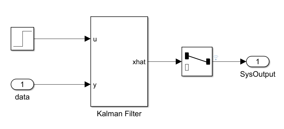
Signal filtering in Simulink using the built-in Kalman Filter unit
Model analysis
Let's analyze the model simulinkKalmanFilter.slx:
Block Settings Kalman Filter:
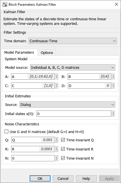
To the input port data models simulinkKalmanFilter.slx the values of the noisy signal are transmitted noisy from the model juliaCodeIntegration.engee due to this, the filtered signals obtained in the two simulation environments can be compared.
Running the simulation
Extracting the variables time and data required to run the simulation in Simulink, from the file juliaCodeIntegration_noisy.csv received after completion of the simulation in Engee:
mat"""
skf_T = readtable('/user/CSVs/juliaCodeIntegration_noisy.csv', 'NumHeaderLines', 1);
time = skf_T.Var1;
data = skf_T.Var2;
"""
Let's model the system:
mdlSim = joinpath(demoroot,"simulinkKalmanFilter")
mat"""myMod = $mdlSim;
    out = sim(myMod);""";
Simulation results
Importing the simulation results:
skf_data = mat"out.yout{1}.Values.Data";
skf_time = mat"out.tout";
Let's build a graph:
plot(juliaCodeIntegration_noisy_t, juliaCodeIntegration_noisy_y, label = "The original signal")
plot!(skf_time, skf_data, label = "Filtered signal")

title!("Signal filtering in Simulink (Kalman Filter)")
xlabel!("Time, [s]")
ylabel!("Angular position of the pendulum")
Comparison with the result obtained in Engee
Let's determine the average absolute error of calculations:
tol_abs = skf_data - juliaCodeIntegration_filtered_y;
tol_abs_mean = abs(mean(tol_abs))
Let's determine the average relative error of calculations:
tol_rel = (skf_data - juliaCodeIntegration_filtered_y)./skf_data;
tol_rel_mean = abs(mean(filter(!isnan, tol_rel))) * 100
Let's plot the absolute error of calculations.:
plot(skf_time, broadcast(abs, tol_abs), legend = false)

title!("Comparison of the results obtained in Engee and Simulink")
xlabel!("Time, [s]")
ylabel!("Absolute error of calculations")
Based on the results obtained, it can be concluded that the implementation of the Kalman filter using
The Engee Function block is not inferior in accuracy to the Kalman Filter block built into Simulink.
Conclusions
This example demonstrates how to integrate Julia code into Engee models and the features of using the Engee Function block - working with multidimensional signals, transferring parameters, and connecting external source code files.