Engineering data and signals
# import Pkg
# Pkg.add(["Statistics", "StatsBase", "StatsPlots", "CSV", "DataFrames", "Dates", "XLSX", "MAT", "WAV", "Images", "FileIO", "DSP", "FFTW", "DelimitedFiles"])
Importing libraries
We'll connect libraries for working with data, signals, and visualization. StatsBase and Statistics will provide statistical functions. CSV, XLSX, and MAT will allow you to read data from the appropriate formats. WAV is for audio files. Images - for uploading images. DSP and FFTW are for spectral analysis.
using Statistics, StatsBase, StatsPlots
using CSV, DataFrames, Dates, XLSX, MAT, WAV, Images, FileIO
using DSP, FFTW, DelimitedFiles
include("media_player.jl")
Reading a CSV file with energy consumption data
Let's start with the most common engineering data format, CSV. Let's read the file with the energy consumption indicators of the steel company. The CSV.read function returns a DataFrame, a tabular structure where columns are available by name. We will immediately deduce the dimension in order to understand the scale of the data.
df_energy = CSV.read("Steel_Industry.csv", DataFrame)
println("Data dimension: ", size(df_energy))
println("Column Names: ", names(df_energy))
Initial data inspection
The first rule of an engineer when receiving data is to look at it through his eyes. We will display the first and last rows, column types. This will help to detect problems: omissions, incorrect types, unexpected values.
println("The first 10 lines:")
first(df_energy, 10)
println("\Column data types:")
[names(df_energy) eltype.(eachcol(df_energy))]
Date and time conversion
In engineering data, timestamps are often stored as strings. Converting the date column to the DateTime format. After the conversion, we can calculate the date range and the average measurement step. Add a new DateTime column to the DataFrame.
df_energy.DateTime = DateTime.(df_energy.date, dateformat"dd/mm/yyyy HH:MM")
println("Range: ", minimum(df_energy.DateTime), " — ", maximum(df_energy.DateTime))

step_sec = mean([Dates.value(dt)/1000 for dt in diff(df_energy.DateTime)])
println("The middle step: ", round(step_sec, digits=2), " sec")
Visualization of a time series
A graph is the best way to understand the behavior of a system. Let's plot the energy consumption for the entire period. On the X-axis is time, on the Y - kilowatt-hours. We see cyclical patterns and outliers.
plot(df_energy.DateTime, df_energy.Usage_kWh,
     xlabel="Time", ylabel="kWh",
     title="Energy consumption",
     linewidth=0.5, legend=false, size=(900, 350))
Reading data from a MAT file
The MATLAB (.mat) format is a standard in engineering practice. It can store signals, matrices, and structures. Let's read the file with the acoustic signals of the bearing. The matread function returns a dictionary, where the keys are variable names and the values are matrices.
подшипник = matread("Bearing.mat")
println("The keys are in the file: ", keys(подшипник))
println("The signal size is normal: ", size(подшипник["normal"]))
Converting MAT data to a vector
The data from the MAT file is stored as 1×N matrices. We transform them into one-dimensional vectors using the vec function. Now it's a regular Julia array of numbers that you can perform mathematical operations with.
норма = vec(подшипник["normal"])
ролик = vec(подшипник["roller"])
println("Data type: ", typeof(норма))
println("Signal length: ", length(норма))
println("\The first 5 samples of the normal signal: \n", норма[1:5])
Reading a WAV audio file
Acoustic data is often stored in audio formats. The wavread function returns an array of samples and the sampling rate. Unlike MAT, here the data is immediately represented as a vector.
сигнал_wav, fs_wav = WAV.wavread("Bearing_1.wav")
println("Sampling rate: ", fs_wav, " Hz")
println("Duration: ", round(length(сигнал_wav)/fs_wav, digits=2), " sec")
Audio file playback in Engee
We will reproduce the acoustic signal of the bearing using the built-in audio player.
media_player("$(@__DIR__)/Bearing_1.wav", mode="audio")
Spectral analysis via FFT
The fast Fourier transform translates the signal from the time domain to the frequency domain. It is a key tool for vibration and acoustic analysis. We center the signal, apply FFT, and take the module for the amplitude spectrum. We will plot only the first half (frequencies from 0 to Nyquist).
signal = normal[1:4000] .- mean(norm[1:4000])
spectrum = abs.(fft(signal))
N = length(signal)
frequencies = (0:N÷2-1) * 10000 /N

plot(frequencies, spectrum[1:N÷2],
     xlabel="Frequency, Hz", ylabel="The amplitude",
     title="Acoustic spectrum of the bearing",
     linewidth=1, legend=false, size=(800, 350))
Data compression via FFT
One of the practical tasks is data compression. Let's look at the spectrum and determine in which range the main energy of the signal is concentrated. Then we will leave only a few key frequency components - this will be a compressed representation. Instead of 4000 signal samples, you can store 20 numbers.
amplitudes = spectrum[1:N÷2]
energy_in total = sum(amplitudes.^2)
cum_energy = cumsum(amplitudes.^2) / General energy

plot(frequencies, cumulation_energy,
     xlabel="Frequency, Hz", ylabel="Stored energy",
     title="Cumulative energy of the spectrum",
     linewidth=2, legend=false, size=(800, 350))
hline!([0.95], linestyle=:dash, label="95% of the energy")
Selecting informative frequency bands
Let's divide the frequency range into 20 equal bands and calculate the average amplitude in each. This will give a compact representation of the signal - 20 numbers that can be stored in a table.
track_strip = 20
stripes = range(0, 5000, length=col_strip+1)
sign_fft = zeros(color_strip)

for i in 1:col_strip
    mask = (frequencies .>= bands[i]) .& (frequencies .< bands[i+1])
    if sum(mask) > 0
        sign_fft[i] = mean(amplitudes[mask])
    end
end

bar(1:color_strip, sign_fft,
    xlabel="Band number", ylabel="Average amplitude",
    title="Compressed signal representation (20 bands)",
    legend=false, size=(700, 300))
Reading an image
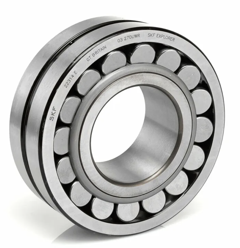
Let's read the image file. Let's display the image type and its size.
изобр = Images.load("image.png")
println("Image Type: ", typeof(изобр))
println("Size: ", size(изобр))
Let's display the image.
the invention
Converting an image to a numeric matrix
Convert the image into a matrix of numbers.
channels = Float64.(Images.channelview(fig))
channels = permutedims(channels, (2, 3, 1))
The image is represented by a 954×923×4 three-dimensional array. The first two dimensions are 954 rows and 923 columns of pixels. The third dimension consists of four color channels: red, green, blue, and an alpha transparency channel. Each value ranges from 0 to 1, where for color channels 0 means no color, 1 means maximum intensity, and for the alpha channel 1 means full opacity.
Reading a text file with data
Text files are the simplest storage format. Let's read the txt file with numerical data on ambient temperature, determine the number of values, the range, and output the first 5 values.
температура = vec(readdlm("температура.txt"))
println("Number of values: ", length(температура))
println("Range: ", minimum(температура), " ... ", maximum(температура), " °C")
println("The first 5 values: ", температура[1:5])
Reading data from Excel
Excel files are widely distributed in the industry. Similarly, let's read the xlsx file with data on ambient humidity.
xlsx_file = XLSX.readxlsx("влажность.xlsx")
sheet = xlsx_file[1]
# Extract the first column as a vector (skip the header)
влажность = Float64.(лист["A"][2:end])
println("Number of values: ", length(влажность),)
println("Range: ", minimum(влажность), " ... ", maximum(влажность), " %")
println("The first 5 values: ", влажность[1:5])
Data Set Transformation
We transform a data set when some of the original columns are not needed, but new data from external sources needs to be added. Delete the NSM, WeekStatus, Day_of_week, and Load_Type columns, and then add the temperature and humidity columns that were loaded earlier.
select!(df_energy, Not([:NSM, :WeekStatus, :Day_of_week, :Load_Type]))
println("Columns after deletion: \n\n", names(df_energy))
Add previously loaded temperature and humidity variables as new columns. The number of rows must match.
df_energy.Temperature_C = temperature
df_energy.Humidity_Pct = humidity
Let's display the first 10 rows of the updated dataset.
println("The first 10 lines:")
first(df_energy, 10)
Save the converted data set to a new CSV file. The source file Steel_Industry.csv it remains unchanged - all transformations are saved in a new file. Сталелитейные_данные.csv.
CSV.write("Steel_data.csv", df_energy)
Converting a MAT file
The data structure in a MAT file can also be represented in different ways. Suppose we have received 4 bearing data files from the test bench:
- H_1_0.mat – fully functional bearing;
- B_11_1.mat – malfunction of the roller element;
- I_1_1.mat – inner ring malfunction;
- O_6_1.mat – malfunction of the outer ring.
But the data analysis model requires a different structure – one MAT file with four keys "normal", "roller", "inner", "outer", where:
normal – fully functional bearing;
roller – malfunction of the roller element;
inner – malfunction of the inner ring;
outer – malfunction of the outer ring.
Let's upload the first file.
норм_тест = matread("H_1_0.mat")
This file has a different data structure than the required one. Let's display the data.
норм_тест = норм_тест["H_1_0"]
The file has one key "H_1_0, the data in which is a matrix. We know that the acoustic data is located in the second column. We don't need any other data. Let's extract this data.
norm_test = norm_test[:,2]
Let's open the rest of the MAT files.
ролик_тест = matread("B_11_1.mat")
внут_тест = matread("I_1_1.mat")
внеш_тест = matread("O_6_1.mat")
Let's extract the matrices.
ролик_тест = ролик_тест["B_11_1"]
внут_тест = внут_тест["I_1_1"]
внеш_тест = внеш_тест["O_6_1"]
Next, we will extract the second column from each matrix in the same way.
rolik_test = rolik_test[:,2]
intra_test = intra_test[:,2]
vnesh_test = vnesh_test[:,2]
Now we have four vectors with acoustic data.: норм_тест ролик_тест, внут_тест, внеш_тест. They must be assembled into a single MAT file of the previously designated structure. Let's create a dictionary with the necessary keys.
data = Dict(
    "normal" => норм_тест,
    "roller" => ролик_тест,
    "inner"  => внут_тест,
    "outer"  => внеш_тест)
Save this data to a new MAT file.
matwrite("Bearing test.mat", данные)
Let's read the created file.
matread("Bearing test.mat")
The structure of the created file corresponds to the required one. The data is ready for further use.