Exporting a neural network to ONNX format

We create a neural network and save it in ONNX format for future use.

Task description

To deploy a ready-made neural network in the target environment or even embed it in the code for a microcontroller, a common solution is to convert the neural network to a standard, framework-independent ONNX (Open Neural Network eXchange) format.

The most common library for creating and training neural networks in Julia is called Flux. It allows you to create fully connected, convolutional, recurrent neural networks and graphs of other topologies, write your own models of neurons and layers, and training and direct calculation are performed in a compiled, binary form that is as fast as the C language.

The functions for exporting Flux neural networks to ONNX are found in several libraries, but at the moment the most successful is the export tool included in the library. NaiveNAXflux. This library contains tools for interfacing the Flux library with the library for searching for optimal neural network topologies (NAS - Neural Architecture Search). NaiveNAS takes care of working with weights and changing the topology of the neural network, and related packages like NaiveGAflux manage genetic optimization.

We will also install the library. ONNXRunTime, which will allow us to run and test the saved neural network.

Saving a neural network in ONNX

Install the necessary libraries:

Pkg.add(["Flux", "ONNXNaiveNASflux", "ONNXRunTime", "ONNXLowLevel"])

After connecting them, we will be able to export a simple fully connected network to ONNX.:

using Flux
using ONNXNaiveNASflux

# Define the model
model = Chain(
    Dense(784 => 32, relu),
    Dense(32 => 10)
)

# Exporting to ONNX using save()
ONNXNaiveNASflux.save("fc_model.onnx", model, (784, 1));

With the last argument of this command, we specify the dimension of the input data in the format number of features, batch size (features, batch_size).

The number of features in the object description can be obtained from the properties of the Flux neural network, but the size of the batch is not fixed in Flux.

first_layer = model[1]
input_size = size(first_layer.weight, 2)

784

Executing a previously saved neural network

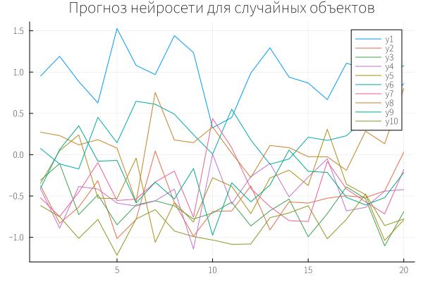
Let's run the saved neural network (the weights in it are initialized with random numbers, so we get noise at the output):

import ONNXRunTime as ORT
fc_model = ORT.load_inference("fc_model.onnx")
fc_model

InferenceSession
    input_names:        ["data_0"]
    output_names:       ["dense_1"]
    execution_provider: :cpu

Now we use the names of the weights to set the inputs and get the outputs from the saved ONNX neural network.:

result = []

for x in eachcol(rand(Float32, 784, 20))
    input_data = Dict("data_0" => reshape(x, 1, :))
    outputs = fc_model(input_data)
    append!(result, [outputs["dense_1"]])
end

gr()
plot(vcat(result...), title="Neural network prediction for random objects")

Exporting other topologies

Here is an export of the main layers of a recurrent neural network with a single RNN layer.

using Flux
using ONNXNaiveNASflux

# This model accepts 5 variables, processes them using RNN, and outputs 2 values.
rnn_model = Chain(
    RNN(5 => 10),      # Inputs: 5 signs, Inner layer: 10 signs
    Dense(10 => 2)     # The output layer translates the state of the hidden layer into two classes/values
)

# Let's define the dimension of the input tensor:
# Variables = 5, Batch size = 1, Input sequence length = 100
input_shape = (5, 1, 100)

ONNXNaiveNASflux.save("rnn_model.onnx", rnn_model, input_shape);

Let's start the recurrent network from the ONNX file:

import ONNXRunTime as ORT
onnx_rnn_model = ORT.load_inference("rnn_model.onnx")
onnx_rnn_model

InferenceSession
    input_names:        ["data_0"]
    output_names:       ["dense_0"]
    execution_provider: :cpu

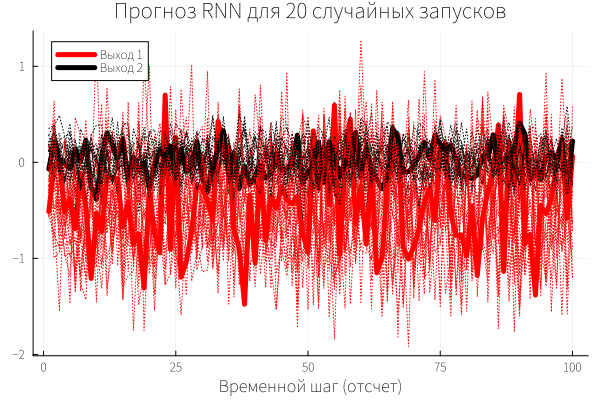
With this information, we can run a recurrent neural network and predict the output features for each sample of the input time series.:

plot()
for x in 1:20
     # We generate a test sequence : 5 signs per 100 samples
     raw_data = rand(Float32, 5, 100)

     # Adding a dimension based on the batch (ONNX standard)
     input_tensor = reshape(raw_data', 100, 1, 5) 
     outputs = onnx_rnn_model(Dict("data_0" => input_tensor))
     onnx_output = outputs["dense_0"]

     # Reassembling the data into a matrix (100 rows, 2 columns)
     plot_data = reshape(onnx_output, 100, 2)

     gr()
     plot!(plot_data, title="RNN forecast for 20 random launches",
         label = (x==1 ? ["Exit 1" "Exit 2"] : false),
         line = (x==1 ? (5,:solid) : (1,:dot)),
         c = [:red :black],
         xlabel="Time step (countdown)")
end
plot!()

Convolutional networks

If you follow the order of the arguments, it's easy to do the same for convolutional neural networks.:

using Flux
using ONNXNaiveNASflux

# A simple convolutional network
# Input: 28x28 (1 channel), Output: 10 classes (for example, numbers 0-9)
cnn_model = Chain(
    Conv((3, 3), 1 => 4, relu), # Convolution: 3x3 filter, 1 input channel, 4 output channels
    Flux.flatten,               # Straightening a tensor into a vector
    Dense(26 * 26 * 4 => 10)    # Fully connected layer for classification
)

# Setting the dimension in the Flux/Julia format: (Width=28, Height=28, Channels=1, Batch=1)
input_shape_cnn = (28, 28, 1, 1)

# Exporting
ONNXNaiveNASflux.save("cnn_model.onnx", cnn_model, input_shape_cnn);

And let's run the convolutional neural network saved in ONNX.:

import ONNXRunTime as ORT

# Loading the model
onnx_cnn_model = ORT.load_inference("cnn_model.onnx")

# 1. Generate a random 28x28 "picture" with 1 channel in Julia (W, H, C) format
# In a real problem, there will be a real image here
raw_image = rand(Float32, 28, 28, 1) 

# 2. Rearranging the axes for ONNX
# From (W=28, H=28, C=1) we make (C=1, H=28, W=28)
permuted_image = permutedims(raw_image, (3, 2, 1))

# Adding the batch dimension to the first position -> we get (Batch=1, C=1, H=28, W=28)
input_tensor = reshape(permuted_image, 1, 1, 28, 28)

# 3. We pass it to the model (the input name for the first layer is usually "data_0")
input_data = Dict("data_0" => input_tensor)
outputs = onnx_cnn_model(input_data)

# 4. Extract the output data
# The output will be a tensor with logits (probabilities) for 10 classes
onnx_output = outputs["dense_0"]

# 5. We forcibly reduce to a one-dimensional vector (10 elements) for the graph
# This will protect us from any output batch structure (be it 1x10 or 10x1)
plot_data = reshape(onnx_output, :)

# Visualization of the forecast for 10 classes
gr()
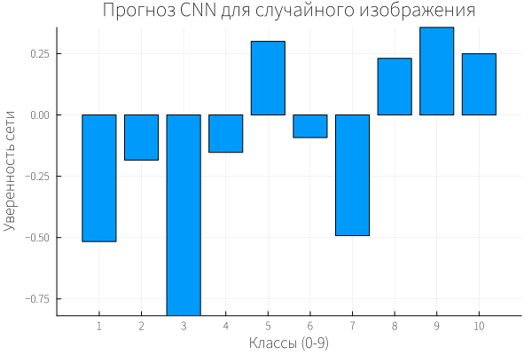
bar(plot_data, title="CNN forecast for a random image", 
    xticks=1:10, xlabel="Grades (0-9)", ylabel="Network Confidence", legend=false)

Conclusion

We figured out how to save three main types of neural networks in ONNX. Not all constructions from Flux are exported reliably, or even have support in ONNXNaiveNASflux. Experimentation and simplification of your topology may be required.