Implementation of the Nyquist filter for pulse signal processing

In modern digital communication systems, the quality of information transmission directly depends on the efficiency of signal processing, where formative filters play a key role. Among them, filters with root Raised Cosine (RRC) are of particular importance, which provide an optimal compromise between spectral efficiency and resistance to Intersymbol Interference (ISI). These filters have become the de facto standard in most modern communication systems, including 5G cellular networks, satellite communications, and high-speed modems.

However, designing RRC filters is a complex engineering task that requires taking into account many parameters: the roll-off factor, the filter length in characters, the number of samples per character, and the accuracy of data representation. The traditional approach to developing such filters involves a laborious iterative process, including calculating coefficients, choosing an implementation structure, optimizing bit depth, and verifying characteristics. Adding particular complexity is the need to take into account the effects of quantization when moving to a fixed-point hardware implementation.

This article demonstrates the practical implementation of the method using the example of an RRC filter with a smoothing coefficient of 0.2, a length of 10 characters and 8 samples per character, including a comparative analysis of direct and transposed structures, verification of frequency and time characteristics.

Let's move on to development, the code below calculates the coefficients for the FIR filter with root cosine characteristic (RRC), which is the main shaping filter in modern digital communication systems. Function rrcosfilter calculates the impulse response of the filter based on the specified parameters: the roll-off factor smoothing coefficient, the length of the filter in characters, and the number of samples per character. The filter ensures optimal formation of the spectrum of the transmitted signal, minimizing intersymbol interference and limiting the frequency band. Calculation of coefficients is the first stage of filter design and its basis.

The direct form of the FIR filter is a classical implementation structure of a finite pulse filter in which the input signal sequentially passes through a chain of delay elements, each output of which is multiplied by the corresponding filter coefficient, and the results are summed to produce an output signal.

Code Description:

This code automatically creates a model of the direct form of the FIR filter based on the previously calculated RRC coefficients. First, a unique model name is generated and a fixed-point format with 16 bits and 14 fractional digits is determined. The coefficients are converted to a fixed point format.

Then, a filter structure is created in the loop: for each coefficient, Gain, Delay, and Addition units are added. A chain of delay elements is formed, where each delayed signal is multiplied by the corresponding coefficient and summed with the previous results. The first coefficient processes the current input signal, and subsequent coefficients process delayed versions of the signal.

The input signal is applied simultaneously to the first gain element and the first delay, creating a cascade structure. All mathematical operations are performed in a fixed-point format to ensure compatibility with the hardware implementation. After building the complete structure, the model is saved to a file and uploaded for further use, providing automated creation of the filter architecture with minimal developer intervention.

The transposed form of the FIR filter is an alternative implementation structure in which all multiplication operations by coefficients are performed in parallel with the input signal, and the results are sequentially accumulated through a chain of adders and delay elements.

Code Description:

This code creates a transposed FIR filter structure, which is fundamentally different from the straight form. In this architecture, the input signal is simultaneously applied to all the multiplication units (Gain), each of which multiplies it by the corresponding coefficient. The resulting products are then sequentially summed through a chain of adders, between which delay elements are inserted. This creates pipelining, where data flows through the entire structure every clock cycle.

Advantages of the transposed form for Verilog code generation:

1. Minimum critical delay — the path from input to output contains only one adder and one delay element, which allows you to achieve a higher clock frequency
2. Natural pipelining — The structure is ideal for conveyor processing, increasing throughput
3. Parallel multiplication — all multiplication operations are performed simultaneously, which simplifies parallelization of calculations in hardware
4. Simplified routing — it is easier to implement a parallel structure with a single data source in FPGAs
5. Better scalability — Adding new coefficients does not increase the critical path

For Verilog code generation the transposed form is preferable because it directly corresponds to the high-frequency hardware implementation with pipelining, providing better time performance and more efficient use of FPGA resources while maintaining functional equivalence with the direct form.

In the course of the work, the interpolation and decimation process for a single pulse was implemented. The initial impulse was set by the vector impulse = [1.0; zeros(100)] which was then convoluted with the filter coefficients coef to generate the transmitted signal tx_signal.

On the receiving side, the reverse operation was performed — the convolution of the received signal with the same coefficients, which gave the reconstructed signal. rx_signal. Visualization of the results — plotting the initial pulse, interpolated and decimated signals — showed their high similarity, which confirmed the correctness of the algorithm implementation.

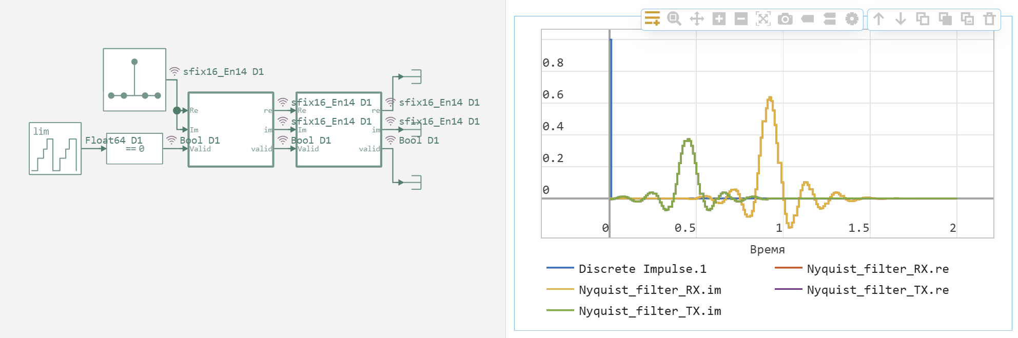
A similar procedure was successfully reproduced in the model using the algorithms implemented by us for validations, which additionally verified the correctness of the approach. The resulting model is a ready-made solution suitable for generating code in the Verilog language.

The generated Verilog code is a hardware implementation of Nyquist transmitting (TX) and receiving (RX) filters for pulse signal processing. Main components:

1. Top-level modules (one_impulse_Nyquist_filter_TX/RX.v):

   • Manage data synchronization and validation
   • Contain a finite state machine for data flow control
   • Integrate FIR filter and delay unit
   • Both filters use the same processing cores (FIR and Delay), but they differ in control logic and activation conditions.

2. FIR filter (fir_liner_1.v):

   • Implements a linear FIR filter (41 coefficients)
   • Uses fixed coefficients to generate an impulse response

• Processes signed 16-bit data

3. Delay unit (Delay_40.v):

   • Implements a chain of 40 delay registers
   • Synchronizes a valid signal with a filtering delay
   • Provides temporary data reconciliation

Conclusion

The simulation confirmed the correctness of the pulse processing implementation. The similarity of the results obtained in the mathematical environment and the hardware model proves the correctness of the algorithm and the accuracy of the selected filter coefficients.

The successfully generated hardware code represents full-fledged transmitting and receiving modules. They are built on a common filter core and differ only in control logic, which ensures energy efficiency of transmission and continuity of reception. The code is modular and ready for synthesis for implementation on the target digital platform.