Sigma-delta ADC of the 4th order
This is a high-precision analog-to-digital converter (ADC) which achieves exceptional resolution (often 16-24 bits or more) due to two key techniques:
-
A heavily roughened but very fast 1-bit ADC (comparator) inside.
-
Complex digital filtering of the 4th order, which "catches" a useful signal from the huge amount of noise generated by this crude ADC.
The "4th order" indicates the degree of complexity and effectiveness of the internal noise reduction system.
Sigma-delta ADC of the 4th order is a tool for precision measurements:
-
Precision measuring instruments: Multimeters, spectrum analyzers.
-
Slow telemetry and sensors: Temperature, pressure, and load sensors (strain gauges), especially in industrial and medical devices.
-
High-end audio equipment (Hi-Fi, studio equipment): For digitizing audio with minimal distortion.
-
Weighing: Commercial and laboratory scales of the highest class.
-
Seismic exploration and geophysics: Where recording of weak low-frequency signals is needed.
You can learn about the principles of operation of the "basic" sigma-delta DAC of the first order in this примере. And read [this article](https://kit-e.ru/delta-sigma-modulyacziya-nazad-v-budushhee /) for a deeper understanding of its working principles.
In this project, we will look at a dynamic model of a more complex analog-to-digital converter circuit, and compare two types of low-pass decimating filters used in similar devices.
ADC Structure
Consider the upper level of the SDADC_4thORD.engee model:
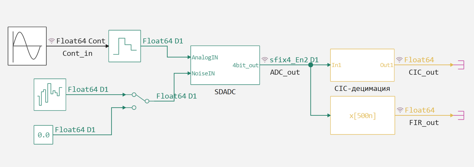
A continuous sine wave unit is used as the source of the test signal, which generates two periods over a time interval of 0.02 seconds - that is, the main oscillation frequency is 100 Hz. This signal then undergoes a sampling operation with a frequency of 1 MHz.
Choosing such an inflated sampling rate is standard practice when using a sigma-delta ADC. In this case, to successfully restore a signal with a fundamental frequency of 100 Hz, it would be enough to take its discrete samples with a frequency of at least 200 Hz. But in the considered model, in order to preserve the relatively smooth shape of the digital sinusoidal signal, it was decided to take a margin 10 times higher than the requirement of Kotelnikov's theorem, that is, the output sampling frequency of the signal should be 2 kHz.
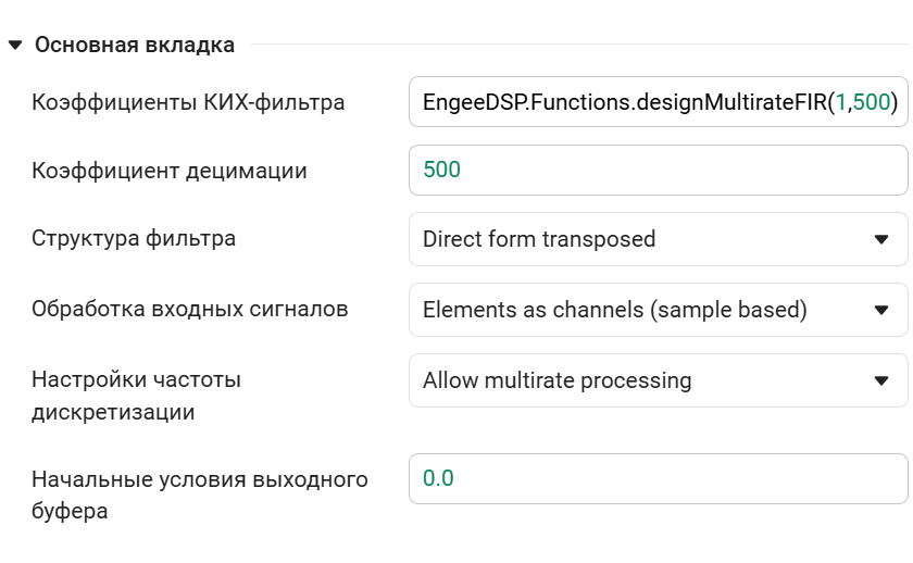
Therefore, immediately after the output of the SDADC block, the signal with a bit depth of 4 bits and a sampling frequency of 1 MHz gets to the decimators, which are based on the CIC filter and FIR filter. Both of these circuits reduce the sampling rate of the signal by 500 times. Parameters of the FIR decimator unit:
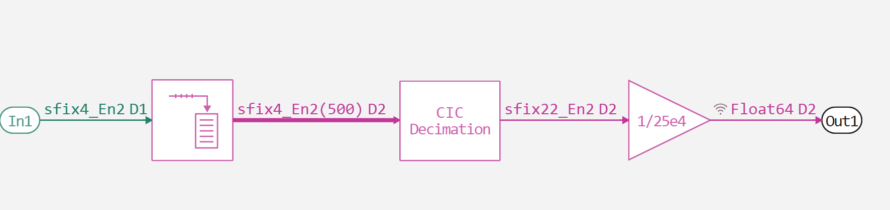
And the structure of the CIC-decimator subsystem:
4th order converter circuit
The SDADC subsystem contains a generalized structure of the 4th order converter with the possibility of modeling additive noise:
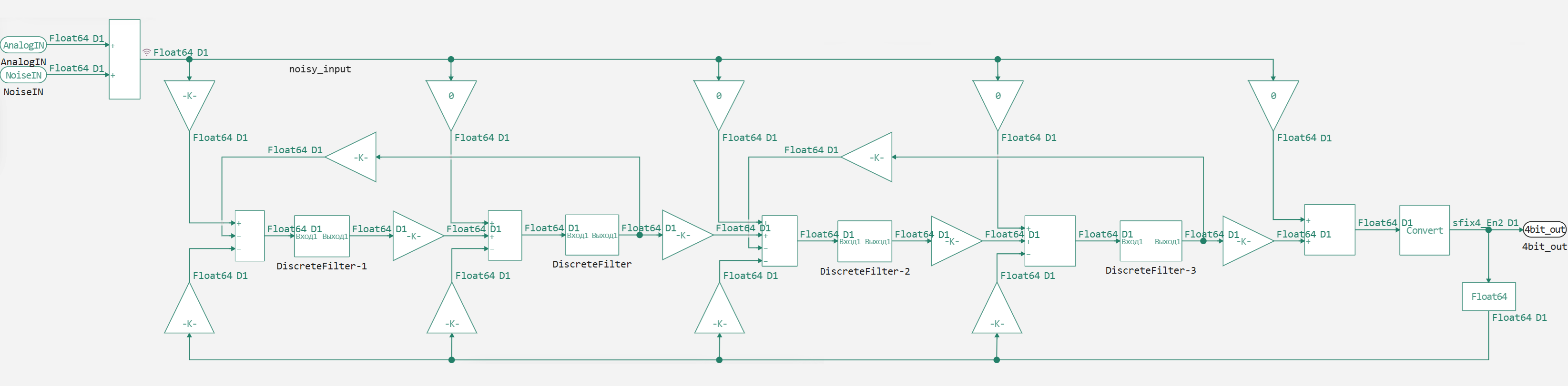
In this case, the "Data Type Conversion" block is used as a quantizer at the output of the circuit, which outputs a signed four-bit signal. White noise with a limited bandwidth can also be applied to the circuit to assess the effect of signal distortion on the digitization result.
Simulation of the model
When running the model for dynamic simulation in the "Signal Visualization" window, you can observe both a continuous input signal and a comparison of the outputs of two decimating filters.:
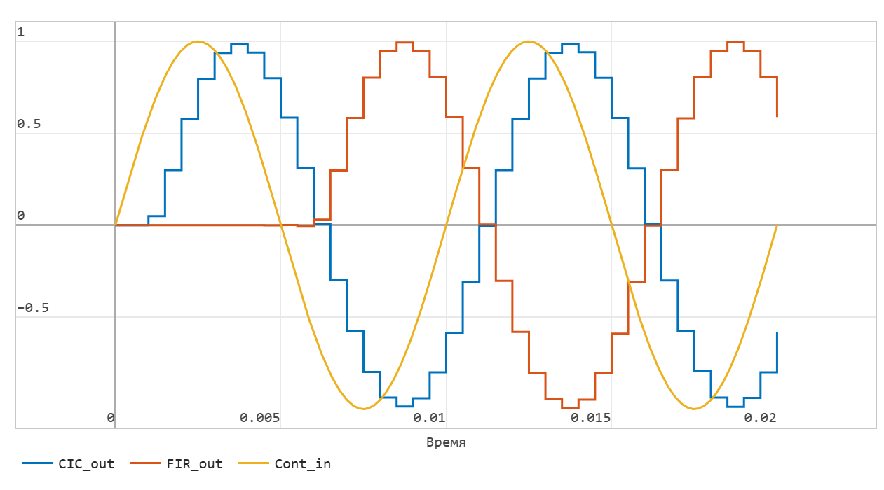
We see that the FIR filter of such a large order introduces a significant delay, but the shape of the discrete sinusoids is identical.
Programmatic analysis of simulation results
Let's run the model programmatically and analyze the logged signals in the time and frequency domains. Saving all the signals to the result variable:
demoroot = @__DIR__
mdl = engee.open(joinpath(demoroot,"SDADC_4thORD.engee"))
result = engee.run(mdl);
We will display the noisy input and the four-bit output of the SDADC subsystem in time.:
noisy_input = collect(result["noisy_input"]);
ADC_out = collect(result["ADC_out"]);
plot(ADC_out.time,ADC_out.value,l=:steppost, label="ADC_out")
plot!(noisy_input.time,noisy_input.value,lw=3, label = "noisy_input")
An interesting feature in the signal spectrum at the output of such a circuit is that the noise generated by the roughness of 1-bit quantization does not disappear, but ** the shape of the spectrum of this noise is changed** by the feedback system. It is "pushed out" (suppressed) in the low-frequency part of the spectrum and amplified at high frequencies. Since our useful signal is low—frequency, the digital filter easily cuts out this shifted high-frequency noise.
Consider the ADC_out signal in the frequency domain:
using EngeeDSP.Functions
p,f = pspectrum(ADC_out.value,1e6);
plot(f,10log10.(p),title="The spectrum at the output of a 4-bit ADC")
And consider the spectrum of the signal at the output of the decimating CIC filter.:
CIC_out = collect(result["CIC_out"]);
periodogram(CIC_out.value, NFFT = 2048, fs = 2e3)
Conclusion
We examined the sigma-delta ADC model of the 4th order, which uses a 4-integrator structure and digital filtering to achieve a record accuracy/cost ratio in applications where the purity and resolution of the digitized low-frequency signal is not important.