Spectrum Analyzer spectrumAnalyzer
The EngeeDSP library includes an advanced tool for evaluating and visualizing signal spectra, the spectrumAnalyzer system object. Let's look at the basic scenarios of its application for the tasks of spectral analysis of various signals, and also learn how to change the parameters of an object.
Methods of spectrum estimation
In this section, we will get acquainted with the main parameters of the EngeeDSP.spectrumAnalyzer object, and, in particular, with the available spectrum estimation methods - the filter bank and the Welch method.
The first test signal:
First, let's create a test signal. x for analysis. This is the sum of two sinusoids and Gaussian noise. Sampling rate of the signal Fs It is equal to 20 MHz, the main frequencies of sinusoids are 2 MHz and 4 MHz (a sinusoid with a higher frequency has an amplitude of 0.25). It is also important to note that for the analysis we chose a signal with a duration of nsamp = 40,000 counts.
Fs = 20e6;
dt = 1/Fs;
nsamp = 40000;
t = 0:dt:(nsamp*dt)-dt;
f1 = 2e6;
f2 = 4e6;
x = sin.(2*pi*f1*t) .+ 0.25*sin.(2*pi*f2*t) + randn(length(t));
plot(t,x, xlim = (0,t[200]), leg = false)
Let's make sure that the signal fluctuates around zero throughout its entire length. Using the function std libraries EngeeDSP:
EngeeDSP.Functions.std(x)
We are observing a mathematical expectation close to zero.
The spectrumAnalyzer System Object
Creating a system object scope1 type EngeeDSP.spectrumAnalyzer. We will explicitly specify some of the parameters, namely the sampling rate. SampleRate and the spectrum representation (one-sided). We will leave the other parameter values by default.
scope1 = EngeeDSP.spectrumAnalyzer();
scope1.SampleRate = Fs;
scope1.PlotAsTwoSidedSpectrum = false;
scope1
An extensive list of parameters available for modification is displayed, but for now we will note the parameter of the spectrum estimation method. Method = "filter-bank", the display type is "power spectrum" SpectrumType = "power", ViewType = "spectrum", as well as setting the frequency resolution RBWSource in the value "auto".
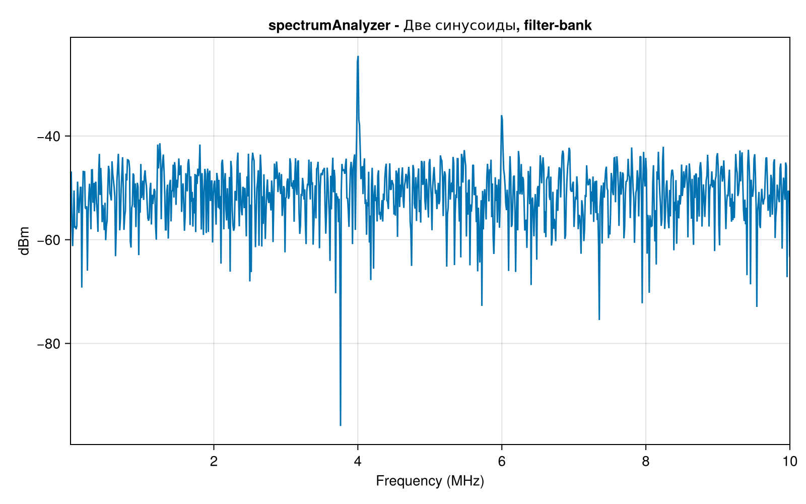
If you apply for the "input" of a variable scope1 our test signal x, then a graph of the signal power spectrum is automatically displayed. By the way, the name of the graph and the axis labels are also parameters of the system object. Setting the field value Title, and call the object:
scope1.Title = "spectrumAnalyzer - Two sinusoids, filter-bank";
scope1(x)
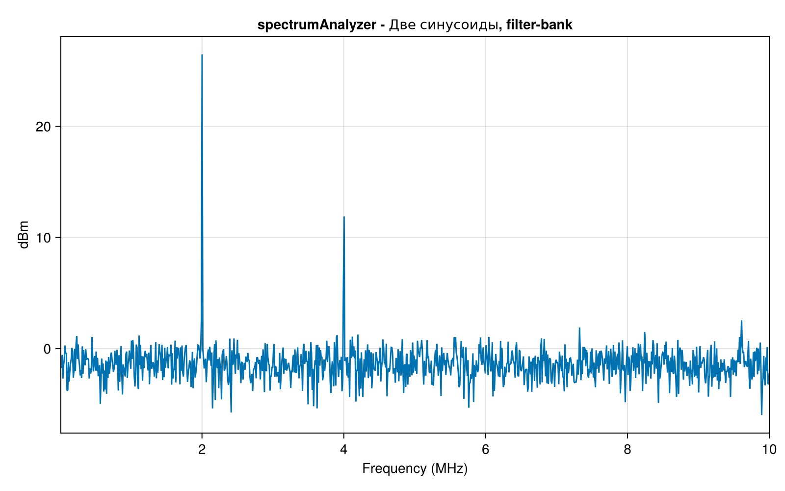
A filter bank is a set of multiple filters (usually bandpass filters) that cover the entire frequency range under study. Many real-world devices, spectrum analyzers, use filter banks to split the signal into multiple frequency bands. This allows you to analyze the signal spectrum in more detail, since it is divided into subchannels (in the analysis bank), and then can be restored (in the synthesis bank).
You can read more about the method [here] (https://kit-e.ru/bank-czifrovyh-filtrov /).
Recording of spectrum samples in a variable
Function getSpectrumData allows you to get numerical samples of the spectrum values in the form of a vector or matrix. To the dictionary spectrumdata we will place the values of frequencies and samples of the power spectrum. Then we will display the spectrum using variables f1 and s1 on a standard graph, the function plot. Now we can interactively and programmatically evaluate the power level and the position of the peaks corresponding to the test sinusoids.:
spectrumdata = EngeeDSP.getSpectrumData(scope1);
f1 = spectrumdata["frequencies"];
s1 = spectrumdata["spectrum"];
plot(f1,s1,leg=false)
The Welch method
The Welch method is one of the basic methods for estimating the signal spectrum based on the fast Fourier transform (FFT). It is widely used for most spectral analysis tasks, especially when processing does not take place in real time and ease of configuration is important.
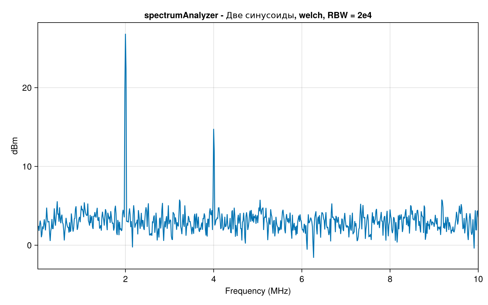
Let's create another system object of the spectrum analyzer scope2 but this time we will specify the Welch method as the main one for evaluation. We will also change the parameters so that we can explicitly control the frequency resolution. RBW, and set its value to 20,000 Hz.
scope2 = EngeeDSP.spectrumAnalyzer();
scope2.SampleRate = Fs;
scope2.PlotAsTwoSidedSpectrum = false;
scope2.Method = "welch";
scope2.RBWSource = "property";
scope2.RBW = 2e4;
scope2.Title = "spectrumAnalyzer - Two sinusoids, welch, RBW = 2e4";
scope2(x)
Let's compare the values of the power spectrum estimates using two methods and display the results on one graph.:
welchdata = EngeeDSP.getSpectrumData(scope2);
f2 = welchdata["frequencies"];
s2 = welchdata["spectrum"];
plot(f1,s1, label = "filter-bank")
plot!(f2,s2, label = "welch", title = "Comparison of methods")
By changing the frequency resolution when using the Welch method, you can also observe a change in the noise level. And when using the filter bank method, it is important to monitor the duration of the signal, and when short "segments" arrive, accumulate them for an accurate assessment of energy.
Spectra of nonstationary signals
Let's use the functionality of the spectrumAnalyzer object to evaluate the spectrum of a signal that varies in its frequency composition over time. A typical signal for such an analysis is frequency modulated.
Let's create a signal whose frequency increases linearly over time, that is, a signal with linear frequency modulation (LFM). To do this, use the function chirp from the EngeeDSP library:
LFM = EngeeDSP.Functions.chirp(t,0,t[end],7e6);
plot(t,LFM, xlim = (0,t[2000]), label = "The LFM signal")
Signal frequency LFM increases linearly from 0 to 7 MHz during the "simulation".
Now let's create another spectrum analyzer object and name it chirpscope. We will set its parameters immediately during initialization in parentheses. Note such parameters as the averaging method and the "forgetting" coefficient, the FFT parameters (number of points, window size), the percentage of overlap for the Welch method, and the type of window function. The resulting graph shape depends on them.
chirpscope = EngeeDSP.spectrumAnalyzer(
    SampleRate = Fs,
    Method = "welch",
    SpectrumType = "power",
    AveragingMethod = "exponential",
    ForgettingFactor = 0.99,
    Window = "hamming",
    WindowLength = 1024,
    OverlapPercent = 75,
    FrequencyResolutionMethod = "window-length",
    FFTLengthSource = "property",
    FFTLength = 1024,
    PlotAsTwoSidedSpectrum = false,
    FrequencySpan = "full",
    ReferenceLoad = 1)
chirpscope.Title = "spectrumAnalyzer - LCHM"
chirpscope(LFM)
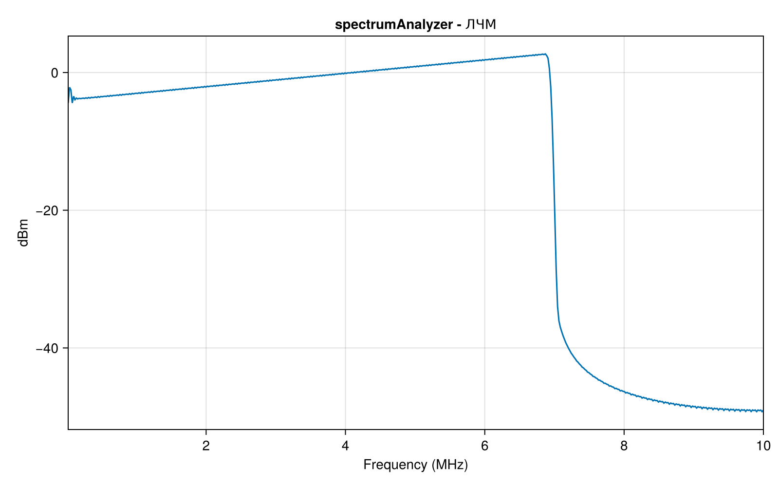
With these parameters, we observe the expected shape of the LFM signal spectrum, it occupies a band from 0 to 7 MHz. However, it is impossible to observe the dynamics of the spectrum change over time on such a graph.
Spectrogram
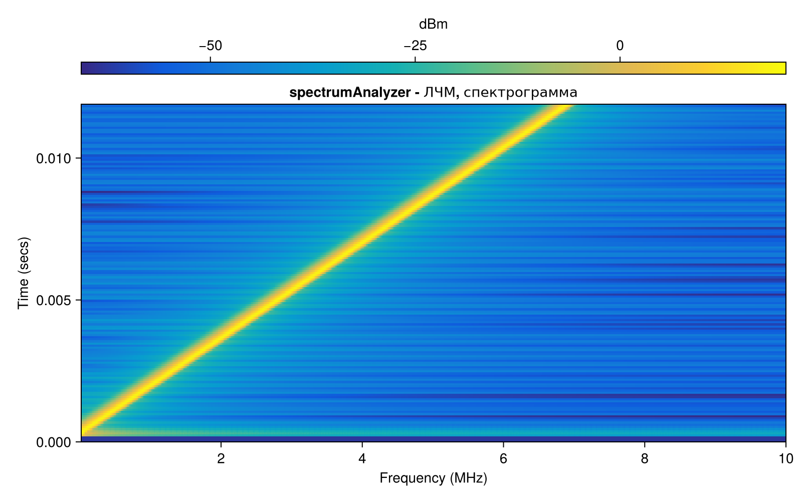
It is useful to use a spectrogram to display the spectra of non-stationary signals in the frequency domain. To do this, we need to change some of the parameters of our object. chirpscope:
release!(chirpscope)
chirpscope.ViewType = "spectrogram";
chirpscope.ForgettingFactor = 0.2;
chirpscope.RBWSource = "property";
chirpscope.RBW = 1e5;
chirpscope.TimeSpanSource = "property";
chirpscope.TimeSpan = 0.012;
chirpscope.Colormap = "parula";
chirpscope.Title = "spectrumAnalyzer - LFM, spectrogram";
chirpscope(LFM)
Accumulation and averaging of the spectrum
When working with streaming signals, techniques for accumulating and averaging spectra calculated on successive time intervals of the signal are used to more accurately assess the energy of the useful spectral components under study and reduce noise. Let's look at this process in dynamics.
The SineWaveDSP system object
Let's create a new test signal, now using another system object of the EngeeDSP library - the sinusoid source SineWaveDSP. This object allows you to sequentially generate segments of an unbroken sinusoidal signal. In our case, we will split the long input signal into segments of 5,000 samples (parameter fSz):
fSz = 5000;

sig1 = EngeeDSP.SineWaveDSP();
sig1.Amplitude = 1;
sig1.Frequency = 4e6;
sig1.SampleTime = 1/Fs;
sig1.SamplesPerFrame = fSz;

sig2 = EngeeDSP.SineWaveDSP();
sig2.Amplitude = 0.25;
sig2.Frequency = 6e6;
sig2.SampleTime = 1/Fs;
sig2.SamplesPerFrame = fSz;

plot(sig1() + sig2() + randn(fSz), xlim = (0,100), label = "SineWaveDSP")
When we analyze a relatively "short" segment of a noisy signal using the filter bank method, we cannot accurately estimate the peak energy, and we also observe a high noise level in the spectrum.:
release!(scope1)
scope1(sig1() + sig2() + randn(fSz))
In real devices, the signal enters the analyzer input sequentially, in precisely such buffered segments, and for a correct assessment it must be accumulated.
The spectrumAnalyzer system object supports various spectrum averaging methods. Let's consider the accumulation with averaging in dynamics. To do this, we will create an animation of sequentially calling system objects of sinusoid sources with additive Gaussian noise, and estimating the spectrum by an object scope1:
release!(scope1)
anim = @animate for i = 1:30
    scope1(sig1() + sig2() + randn(fSz));
    tempdata = EngeeDSP.getSpectrumData(scope1);
    tempf = tempdata["frequencies"];
    temps = tempdata["spectrum"];
    plot(tempf,temps, ylim = (-25,25), leg = false, title = "Spectrum averaging, filter-bank")
end
gif(anim, "spectrum_averaging.gif", fps = 5)
We see a gradual decrease in noise levels, as well as an approximation to an accurate assessment of peak levels.
Conclusion
We got acquainted with the basic functionality of the spectrumAnalyzer system object of the EngeeDSP library. We examined the syntax of its initialization and invocation, the specifics of setting its parameters, and observed their effect on the result of evaluating the spectra of various test signals.