Construction of a spectrogram of a nonstationary complex signal using the FFT block
Let us consider the classical problem of displaying the spectrum of a time-unstable signal. A linear frequency modulation (LFM) signal can be used as such a signal. For example, when the oscillation frequency increases linearly during the simulation. The standard approach of calculating the fast Fourier transform (FFT) of the entire signal during observation will not allow us to estimate the dynamics of the change, which means we need to use the STFT (Short Time Fourier Transform) method to construct a spectrogram, or observe intermediate "frames" of the signal spectrum in dynamics.
Both are easy to implement in the Engee modeling environment using the functionality of the EngeeDSP signal processing library.
Model composition
The dynamic model is assembled in the complex_fft.engee file. We can open it programmatically:
engee.open("complex_fft.engee")
The current model level looks like this:
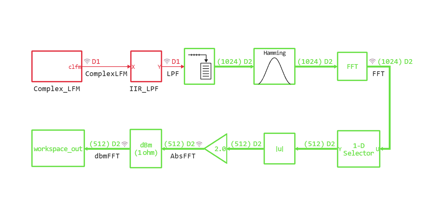
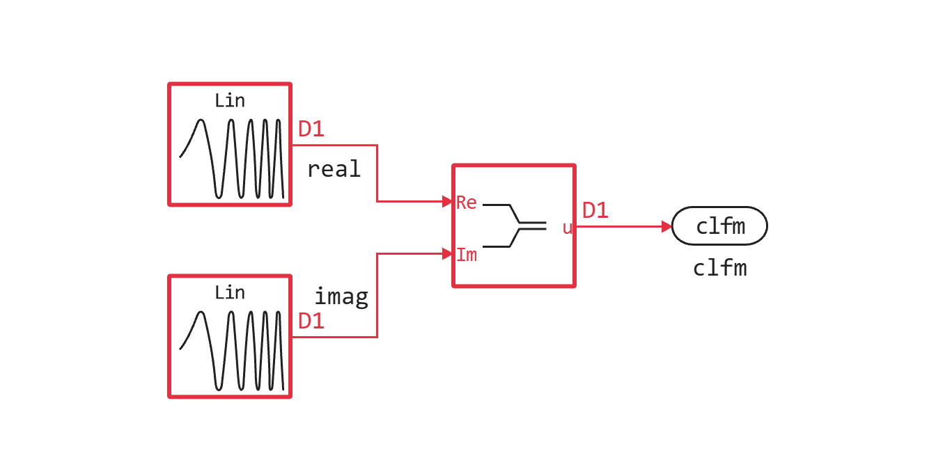
The subsystem Complex_LFM is used as the signal source, in which a complex LFM signal is collected.:
Next, the generated complex signal is sent to a low-pass filter (low-pass filter), which was generated using the Engee interactive application "Digital Filter Editor". The characteristics and specification of the filter in the application are shown in the figure below.:
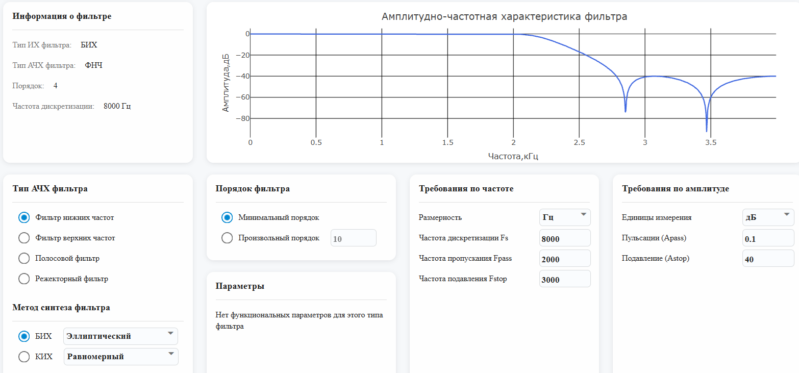
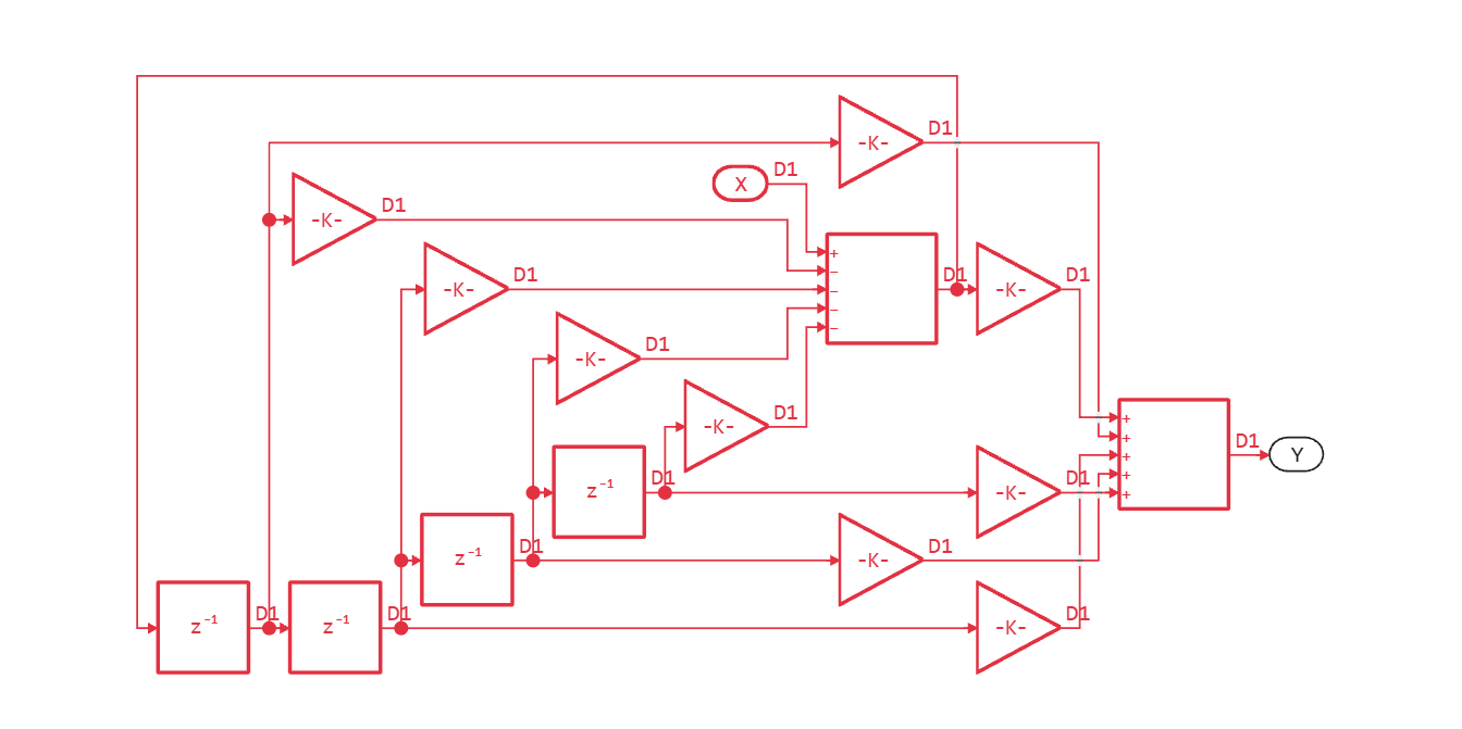
The generated filter structure is located in the IIR_LPF subsystem:
Sequential complex samples after the filter output are sent to the Buffer block, the output of which is a vector of 1024 elements. The Hamming window function is applied to the vector, and then it goes to the input of the FFT block. The subsequent block chain allocates the first half of the output complex vector of FFT samples, calculates the modulus of values, compensates for the energy, and represents the intermediate amplitude spectrum in dBm units.
The results of the run are saved to the workspace_out variable.
Interactive analysis of simulation results
The model is configured in such a way that one second of simulation corresponds to one second of "real" time (wall clock). Thus, after starting the model, in the "Signal Visualization" window, you can observe various outputs in dynamics, both in the time and frequency domains.
Conclusion of the "Signal visualization" window
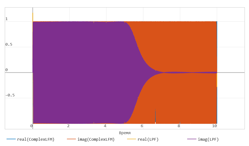
The oscillogram of a complex LFM when passing through the low-frequency looks like this:
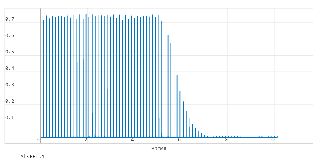
The output of the module of the truncated vector of the FFT output can be observed using the "Frame in the time domain" display type:
The built-in spectrum analyzer of the simulation environment ("Signals in the frequency domain") will display changes in the spectrum of the FM signal before and after the filter in dynamics.:
And the logical output of the "custom" processing chain can also be visualized in dynamics using the "Array construction" option:
Program analysis and spectrogram construction
For the analysis task in the script, we recorded the output of the chain as a block ** In the workspace**. This allows us to represent the frames of the transformation output as a matrix. The model can be run programmatically:
engee.run("complex_fft")
And further in the loop, we will allocate the numerical vectors of the processing results (separate "frames" of the spectrum for the formation of the spectrogram) to the variable outmatrix:
nframes = Int(ceil(stoptime*fs/nfft));
half_nfft = Int(round(nfft/2));
timeline = zeros(nframes);
outmatrix = zeros(half_nfft,nframes);
for k = 1:nframes
    tempvar = workspace_out[k];
    timeline[k] = tempvar[1];
    outmatrix[:,k] = tempvar[2];
end
freqvec = LinRange(0,fs/2,half_nfft);
Let's construct a spectrogram in the form of a three-dimensional surface:
surface(timeline, freqvec, outmatrix, c = :rainbow)
Conclusion
We got acquainted with the functionality of the blocks and interactive tools of the EngeeDSP library for building a dynamic model that processes a non-stationary complex signal. We also considered two ways to visualize the frequency composition of such signals - in dynamics and using a spectrogram.