EngeeDSP System Objects
A system object is a specialized software structure in the Engee technical computing environment. Objects are used to implement and model dynamic systems with time-varying inputs. They simplify the construction of streaming processing systems in Engee scripts.
As an example of a dynamic system, we can consider reading a "frame" of several samples of a signal recorded in a long file, then processing this frame with a digital filter, or spectral analysis using the FFT method or a filter bank. All links in this chain can be represented by a sequence of corresponding system objects.
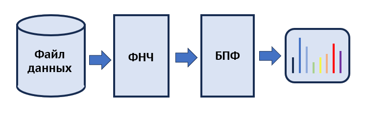
In this example, we will consider the possibility of implementing a streaming processing and visualization scheme similar to the Engee reference model, which was assembled from parameterizable blocks. The reference_FFT.engee model is a variation of the previously discussed model from this примера.
The modified model processes a real signal with linear frequency modulation (LFM) with a low-pass filter (LPF) with a finite impulse response (FIR), and then buffers the data frame and calculates the result of a windowed fast Fourier transform (FFT) followed by visualization of the real part of the spectrum.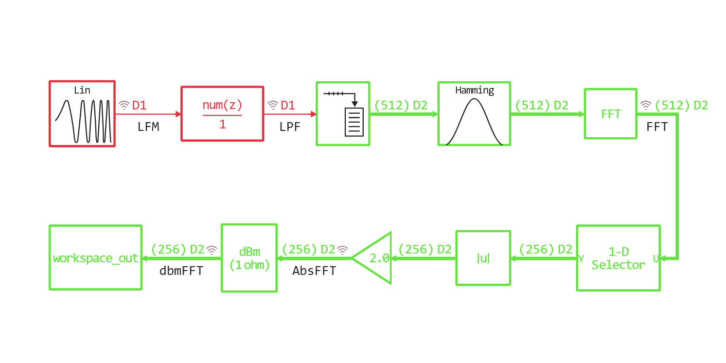
The expected behavior of DSP algorithms can be observed when running the model in the "Signal Visualization" window. We implement this processing chain in a script in the *.ngscript format based on the system objects of the EngeeDSP library.
We will indicate the libraries of system objects and functions of the DSP used.:
using EngeeDSP
using EngeeDSP.Functions
We will set the basic parameters of the digital system, such as the sampling frequency and the size of the processed frame.:
fs = 8000;
framesize = 512;
Source of the streaming signal
We will use the SineWaveDSP system object as a signal source with a linearly varying sampling frequency. It generates a sinusoidal oscillation, the frequency of which we can change in a cycle, thereby approximating the behavior of the FM signal source. We will give him the parameters of the sampling frequency and frame size.:
source = SineWaveDSP();
source.SampleTime = 1//fs;
source.SamplesPerFrame = framesize;
source
Consider the behavior of an object when it is called and states are reset.:
release!(source)
x = source();
plot(x, leg=false)
Low-pass filter
Let's start by prototyping a suitable low-pass filter. To do this, we use the synthesis and analysis functions from the EngeeDSP.Functions library.:
n = 15;
firwin = window("hamming", n+1)
b = fir1(n, 2000/(fs/2), firwin, "low");
freqz(b, 1, 512, fs, out=:plot)
We will transfer the coefficients of the numerator of the transfer function of the filter prototype to the DiscreteFIRFilter system object. The effect of filter states on the shape of the processed signal is described in more detail in [this community example] (https://engee.com/community/ru/catalogs/projects/sistemnyi-obekt-kikh-filtra ):
FIR = DiscreteFIRFilter();
FIR.Coefficients = b;
setup!(FIR, zeros(framesize));
plot(b, l=:stem, m=:c)
Window function
It is not necessary to use a system object for a window function, since its mathematics does not change depending on previous signal values and states. It is enough to simply generate a vector of Hamming window values the size of a data frame in the time domain:
hamwin = window("hamming", framesize);
plot(hamwin,l=:stem,label="Hamming window")
FFT
The EngeeFFT system object will inherit the size of the input frame, but we will divide the numerical values of the complex samples by the length of the FFT.:
FFT = EngeeFFT();
FFT.DivideOutputFFTLength = true;
FFT
Conversion to dBm
The dbConverion object allows you to set the parameters of the input and output signals. In our case, we will convert the amplitude to dBm:
dbconv = dBConversion()
dbconv.ConvertTo = "dBm";
dbconv
The main cycle of accessing system objects
Let's set the numerical vectors of the changing value of the repetition frequency of the sinusoidal signal source freq_range. The frequency will vary from 50 Hz to 4000 Hz in increments of 50 Hz.
We also initialize the frequency grid vector. freqvec for the subsequent display of the spectrum.
The number of iterations of the main loop will correspond to the length of the vector of increasing values of the frequency of the sine wave. The result of processing will be placed frame-by-frame in the matrix spectrum:
freq_range = 50:50:Int(fs/2);
freqvec = LinRange(0.0,fs/2,Int(framesize/2));
count = length(freq_range);
spectrum = zeros(Int(framesize/2),count);
At each step of the cycle, the frequency parameter of the system object of the sine wave generator is changed, and a segment of the sine is recorded in a variable. sine_chunk, processing this frame with an FIR filter, applying a window function, calculating the complex FFT vector, cropping it to the "middle", calculating the modulus and converting it from amplitude to dBm:
for k = 1:count
    source.Frequency = freq_range[k];
    sine_chunk = source();
    LPF = FIR(sine_chunk);
    complexFFT = FFT(LPF .* hamwin);
    absFFT = abs(complexFFT[1:Int(framesize/2)]);
    spectrum[:,k] = dbconv(absFFT);
end
Visualization
Let's display the change in the dynamics of the spectrum over the entire time of the "dynamic simulation" using a three-dimensional surface.:
surface(1:count, freqvec, spectrum)
We also visualize the animation of the spectrum change.:
anim = @animate for i = 1:count
    plot(freqvec, spectrum[:,i],
                    lw=2,
                    ylim = (-120,30),
                    leg = false,
                    title = "The spectrum of the LFM signal",
                    yguide = "dBm",
                    xguide = "Frequency (Hz)",
                    size = (800,200))
end
gif(anim, "dynamic_spectrum.gif", fps = 10)
Conclusion
We have considered the possibility of building a full-fledged dynamic model of streaming processing and visualization of signals based on system objects EngeeDSP. The model includes functional nodes:
- a sinusoid source with a varying repetition rate
- FIR low-pass filter
- Window function
- Fast Fourier transform
- calculations of the signal spectrum in dBm
- visualizations