Sensor multiplexing

How to ensure the reliability of measurements?

Reliable measurements of physical parameters are required in many areas. Such a task cannot be solved with a single sensor, even an ultra-reliable one. To ensure the reliability of measurements, a sensor redundancy approach is used - measurements are carried out by several sensors at once, and their measurements are subject to arbitration. This project will show an example of an arbitration algorithm.

Description of the algorithm

In the simplest case, we could calculate the value as the average of the sum of all sensor readings.:

However, it is necessary to take into account how much we "trust" each sensor. Indeed, if a sensor failure has occurred, then we must take into account that its reliability has decreased. Therefore, each sensor is assigned a weight. , which is taken into account in the calculation:

Sensor simulation

Let's create a sensor model as a noisy sinusoid:

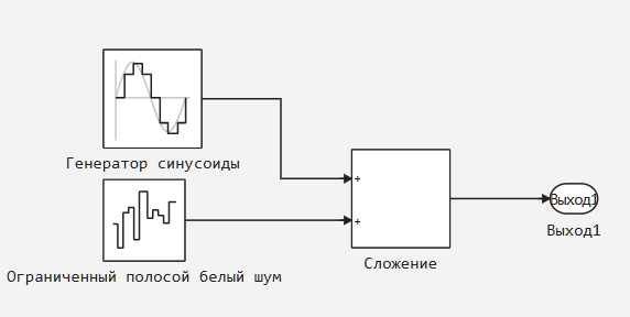
The general model of the system will contain four sensors that detect one "external" signal - a slowly oscillating sine wave. For sensors, we change the parameter of our own additive noise. In addition, it is possible for one of the sensors to simulate a failure in the form of added short-term pulses of large amplitude.

Signal filtering

First of all, you need to suppress your own noise with a digital low-pass filter (low-pass filter). Let's build a spectrogram of our signal using the "Signals in the frequency domain" option in the Signal Visualization section.:

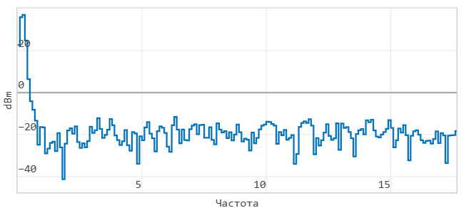
We observe a "useful" low-frequency signal, as well as a noise "bottom", which is expected for additive white Gaussian noise. It is necessary to suppress frequencies above about 2 Hz. Let's use the graphical application "Digital Filter Editor" and create in it a prototype of a digital filter with an infinite impulse response (IIR) and the following parameters:

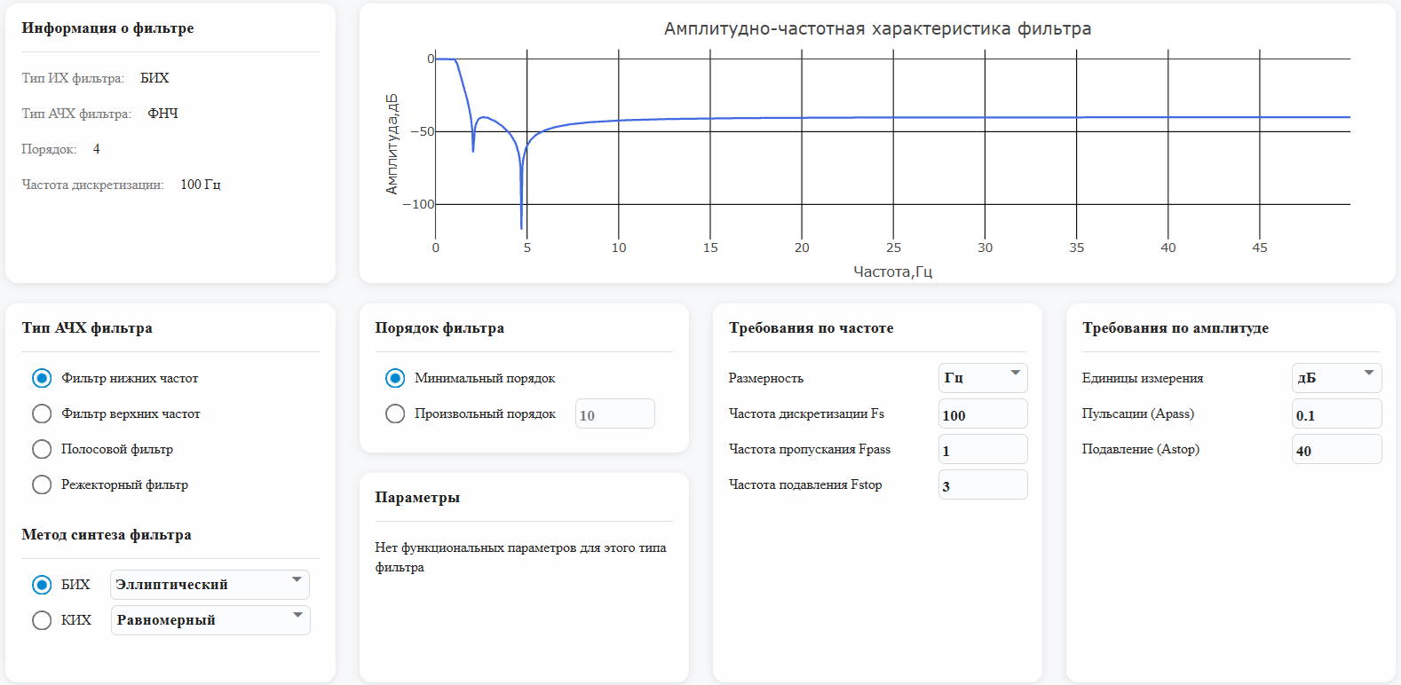
We have seen that the amplitude-frequency response (frequency response) of the resulting filter is suitable for the task of purifying the sine wave from white noise. In addition, the Digital Filter Editor application allows you to automatically obtain the filter structure with synthesized coefficients. This is what the automatically generated IIR filter subsystem looks like.:

The initial signal of one of the sensors and the result of the filter operation are shown below.:

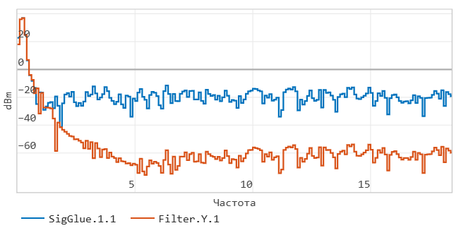
As well as a comparison of the input and output spectra.:

However, the filter cannot cope with smoothing the waveform with high-amplitude outliers. The shape of the sine wave appears to be strongly distorted:

This means that it is necessary to rely on sensor measurements without failures.

Validation of sensor readings

It is necessary to monitor the sensors to see if we can trust the measurement. The control will be carried out according to two criteria:

1. Is the measurement in the specified range?
2. How fast does the signal change?

The combination of these monitoring methods makes it possible to track most sensor failures.

Let's look at the implementation of this method in the form of the Engee model.:

The signal measurement rate will be monitored by estimating the moving average. If this indicator exceeds the acceptable limits, then this is clearly a measurement error.

Exclusion of emissions

The sensor may be serviceable from the point of view of the monitoring algorithm, but give an inadequate value (for example, after an accident). Such measurements must be detected and excluded from calculations.

As an example, we will measure the temperature with 4 sensors, and we will get the following measurements:

68.8 is a clear outlier! It should be excluded from the calculation. To do this, use the following algorithm: calculate the average of the measurements, and find the deviation from the average. Then we find the standard deviation of the sample and exclude those measurements whose deviation from the mean is greater than the standard deviation of the sample. The implementation of this algorithm is given below.:

This algorithm can be modeled as:

At the output, we will have a bitmask in which 0 means that the sensor should be excluded from the calculation.

Weight management

Earlier, in the description of the algorithm, we introduced the concept of sensor weight. Let me remind you that weight is a measure of confidence in a sensor. Let's assume that after a sensor failure and its subsequent recovery, we begin to trust the sensor less. This means that we have to reduce its weight. Moreover, you can enter a threshold of confidence in the sensor and exclude sensors whose weight is below a certain threshold from the calculation.

Assembling the final model

The final model of the algorithm looks like this:

Here:

• The Filter subsystem is responsible for filtering the signal and was generated by the Digital Filter Editor application.
• The OutlierExclusion subsystem is responsible for eliminating outliers
• The Sensor Validation subsystem is responsible for validating sensors

The algorithm itself is implemented using the Engee Function block.:

mutable struct Block <: AbstractCausalComponent
    sensor_weights::Vector{Float64}
    function Block()
        dims = INPUT_SIGNAL_ATTRIBUTES[1].dimensions;
        new(vec(ones(1,prod(dims))))
        #new(vec(ones(1,4)))
    end

end

function (c::Block)(t::Real, TrustedSensors, sensor_data, SensorValid)
   if t<=0
      return(0.0,c.sensor_weights)
   end
   
   total_weight = sum(c.sensor_weights[TrustedSensors])
   sum_weight = sum(sensor_data[TrustedSensors].*c.sensor_weights[TrustedSensors])
   ret = sum_weight/total_weight;

   if isnan(ret)
      warning("Nan detected with values: TW $total_weight, SW: $sum_weight")
      pause_simulation()
   end

   return (ret,c.sensor_weights)
end

function update!(c::Block, t::Real, TrustedSensors, sensor_data, SensorValid)
    if !isempty(c.sensor_weights[.!SensorValid])
        c.sensor_weights[.!SensorValid] .-= 0.001
    end
    c.sensor_weights[c.sensor_weights .< 0] .= 0
    return c
end
```</span>
{% endcut %}

Please note that the model is already vectorized and can handle any number of sensors. The Sensor Validation subsystem is also of interest. This is a subsystem of the ForEach Subsystem type, which allows you to execute the contents of the subsystem for each element of the vector signal.

Additionally, a weight limit was introduced.

Testing the algorithm

Let's check that our algorithm works. Let's build a test model:

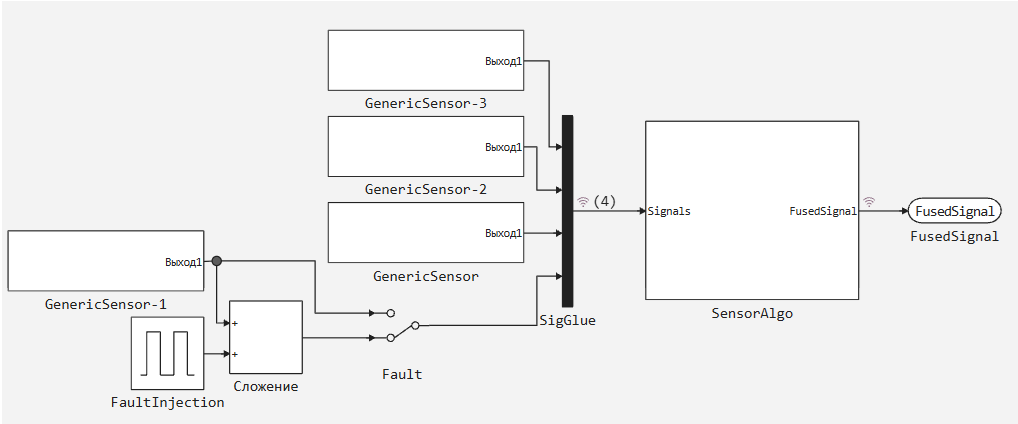
4 sensors are modeled (the sensor model is described above). The failure of the fourth sensor is also simulated. The algorithm model itself is inserted as a reference model.

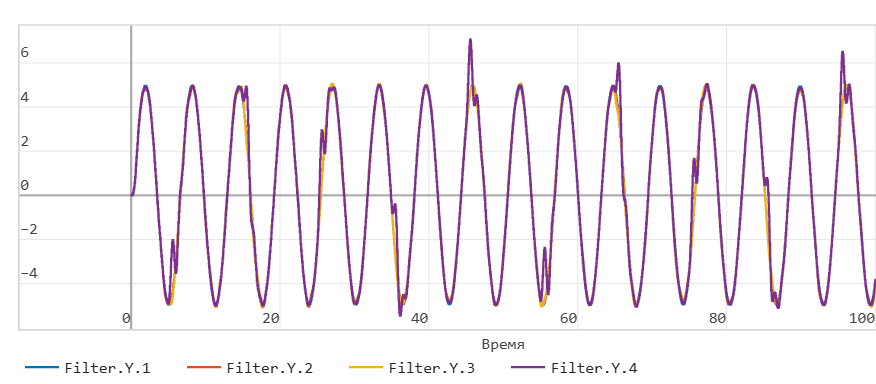
Let's look at the behavior of the algorithm in the absence of failures.:

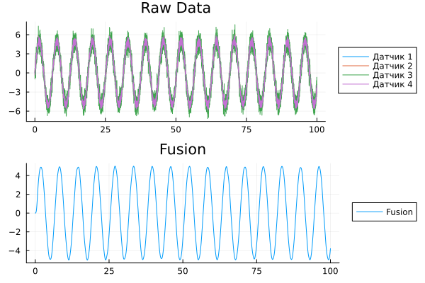
Now let's simulate the failures of the fourth sensor and look at the results.:

It can be seen that the sensor failure did not affect the operation of the algorithm. Thus, we have obtained a fault-tolerant algorithm for measuring a certain value using several sensors.

Conclusion

The project considers a fault-tolerant measurement algorithm and demonstrates a methodologically correct approach to organizing measurements with multiple sensors. As a development of this project, a more detailed sensor model should be considered, taking into account, for example, the accuracy class.