C code from a surrogate neural network
We present a project for a simple generator for fully connected neural networks that allows you to place a neural network in an Engee code block or in a microcontroller.
Environment preparation
Install the necessary libraries:
# Pkg.add(["ChainPlots", "Flux"])
using DataFrames, CSV, Flux, Random, Statistics
using Flux: mse
using ChainPlots
gr();
We collected data for a certain range of input values and saved the output values of the model from the [Fuel Cell System] project (https://engee.com/community/ru/catalogs/projects/sistema-toplivnykh-elementov ) the author shestakoviktor. To study the previous steps, refer to the project Обучение суррогатной нейросети.
We will also need information about inputs and outputs in the current project, so we will repeat the declaration of input and output data.
out_vars = ["Power kW", "Voltage Sensor.V", "The fuel cell.thermal_port.T", "Fuel cell.i_FC"]
v1 = Dict(:block=>"FuelCell/Hydrogen Pressure (bar)",:param=>"Value", :units=>"", :delta=>2.0, :lower=>2.0, :upper=>20.0)
v2 = Dict(:block=>"FuelCell/Fuel supply",:param=>"slope", :units=>"", :delta=>10/60, :lower=>50/60, :upper=>150/60)
adj_vars = vcat(DataFrame.([v1, v2])...)

n_features, n_targets = nrow(adj_vars), length(out_vars)
We have determined the number of input and output variables of our model, and now we can simply download the data from the experiment.
Training a surrogate neural network
Training a neural network on a small amount of data is almost a free procedure, so let's repeat the training, and take only data from the previous project.
include("$(@__DIR__)/scripts/create_plots.jl");
include("$(@__DIR__)/scripts/prepare_data.jl");
include("$(@__DIR__)/scripts/plot_predictions.jl");
l1_neurons = 11 # @param {type:"slider",min:1,max:30,step:1}
l2_neurons = 8 # @param {type:"slider",min:1,max:30,step:1}
l3_neurons = 8 # @param {type:"slider",min:1,max:30,step:1}
l4_neurons = 8 # @param {type:"slider",min:1,max:30,step:1}
l5_neurons = 8 # @param {type:"slider",min:1,max:30,step:1}
n_epochs = 1500 # @param {type:"slider",min:1,max:1500,step:1}
learning_rate_base = 1 # @param {type:"slider",min:1,max:9,step:1}
learning_rate_exp = -3 # @param {type:"slider",min:-6,max:1,step:1}
models_list = []
loss_list = []
loss_plot_list = []
for i = 1:5
include("$(@__DIR__)/scripts/prepare_and_train_net.jl")
append!(models_list, [model])
append!(loss_plot_list, [train_losses])
append!(loss_list, loss(model, X_train_norm, y_train_norm))
end
min_id = findmin(loss_list)[2]
train_losses = loss_plot_list[min_id]
model = models_list[min_id]
best_loss = loss_list[min_id]
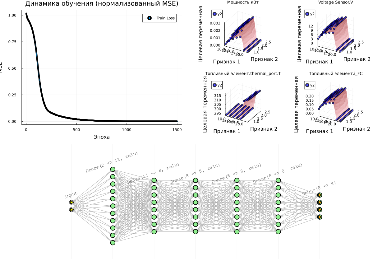
# Graph 1: Learning Curves
p_loss = plot(1:n_epochs, train_losses, label="Train Loss", lw=2, marker=:circle, markersize=2)
title!(p_loss, "Learning Dynamics (normalized MSE)")
xlabel!(p_loss, "Era")
ylabel!(p_loss, "MSE")
println("Received Error value (MSE): ", best_loss)
# Surface graphs for all target variables
surface_plots = [plot_predictions(model, X_train_norm, y_train_norm,
X_train_mean, X_train_std, y_train_mean, y_train_std, i,
title=out_vars[i])
for i in 1:n_targets]
# surface_plots = create_plots(predict_df, :reds, out_var, in_vars, result_df) for out_var in out_vars]
# Displaying all the graphs together
plot(plot(p_loss, plot(surface_plots...)), plot(model), layout=(2,1), size=(1200,900))
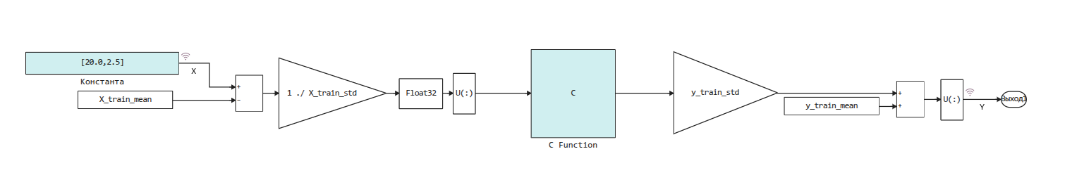
Generating code for a neural network and configuring the model
We have turned the data into an algorithm, and all the coefficients of the model are located in a neural network. model. Since this neural network contains only fully connected layers, it will be easy for us to generate portable C code from it.:
include("$(@__DIR__)/scripts/generate_inline_c_code.jl");
cd(@__DIR__)
engee.open("nnet_model.engee")
engee.set_param!( "nnet_model/C Function", "InputPort1Size" => "($n_features,)")
engee.set_param!( "nnet_model/C Function", "OutputPort1Size" => "($n_targets,)")
engee.set_param!( "nnet_model/C Function", "OutputCode" => generate_inline_c_code(model, n_features, n_targets))
This code is automatically placed in the following model, where the normalization of the input data and the reverse operation for the output data of the algorithm are performed.:
Let's check the resulting model
To test the quality of this neural network directly on the target model, run it on all points of the source table and check the forecasts.:
predict_df = CSV.read("$(@__DIR__)/data/outputfile.csv", DataFrame)
predict_df = filter(row -> all(isfinite, row), predict_df)

in_vars = names(predict_df)[1:n_features];
out_vars = names(predict_df)[n_features+1:end];

for var in out_vars predict_df[!, Symbol(var)] = missings(Float64, nrow(predict_df)); end
After loading the data, all that remains is to create a loop where we will change the block values. Константа and save the results of the model execution.
You can comment out this cell, then the previously saved data will be used.
for row in eachrow(predict_df)
    const_value = "[" * join([string(row[col]) for col in names(predict_df)[1:n_features]], ',') * "]"
    engee.set_param!( "nnet_model/Константа", "Value"=>const_value )
    data = engee.run()
    for (i,var) in enumerate(out_vars) row[Symbol(var)] = data["Y"].value[end][i]; end
end

predict_df = coalesce.(predict_df, NaN);
CSV.write("$(@__DIR__)/data/outputfile_predictions.csv", predict_df);
In order not to run the model repeatedly for each experiment, let's prepare ourselves the opportunity to open the data from the results table and build graphs.:
# Initial training data
result_df = DataFrame(CSV.File("$(@__DIR__)/data/outputfile.csv"))

# Data predicted by the neural network
predict_df = DataFrame(CSV.File("$(@__DIR__)/data/outputfile_predictions.csv"))
p = [create_plots(predict_df, :reds, out_var, in_vars, result_df) for out_var in out_vars]
plot(p..., legend=false, size=(1500,500), titlefont=font(9), guidefont=font(7))
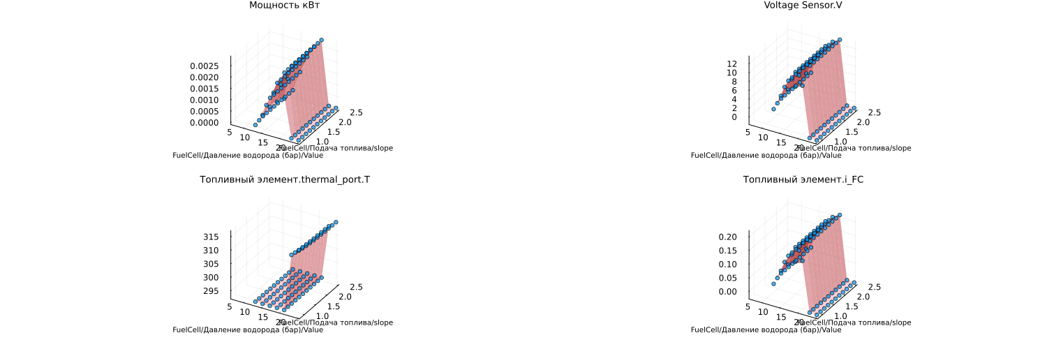
The points on the graph (forecasts) match well with the surfaces obtained after experimenting with the physical model.
Conclusion
We have implemented an approach of transferring a neural network to a block of C code, which will allow us to work with data of any dimension (any number of inputs and inputs of the neural network).
Visualization of results works for two input variables, if there is more data, you should simply limit visualization to two variables or remove it.