Embedded code from a convolutional neural network
Let's train a neural network for a toy task - predicting geometric shapes, and check whether it can be compiled into C code, and then into a binary library to use in blocks or as part of another project.
Introduction
In this practical guide, we will train a neural network to recognize geometric shapes on a toy dataset, and then export the trained model to C code, compile it into a shared library, and test the possibility of integration into third-party projects or C code blocks in your project.
During the conversion, you will notice a slight loss of accuracy. This may be caused by differences in the implementation of some operations in Julia and in C (for example, batch normalization) or simple rounding of coefficients when translated into code, but it opens the way to deployment on embedded systems.
Preparation
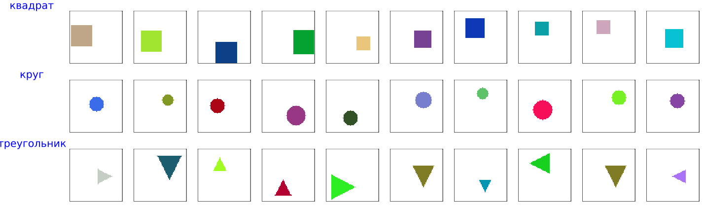
At this stage, we download the necessary libraries, fix a random number generator, create a synthetic dataset of squares, circles, and triangles, and then visualize sample images of each class.
The generation of a controlled, balanced dataset with known properties (64×64 size, normalization to the range [-1.1]) allows you to check each stage of the pipeline in isolation without the influence of external factors.
Let's install the necessary libraries and initialize the random number generator so that our experiment is easily reproducible.:
# Installing the necessary packages
# Pkg.add(["Flux", "BSON", "ImageTransformations"])
using Random
Random.seed!(5);
Synthesizing a data set
Let's create a toy dataset consisting of three classes. Some of the objects are placed in the "unknown" folder, that is, their class, although it is written in the file name, will be unknown to the system. You can call this a validation dataset. The rest - training and test - are arranged in the appropriate folders.
include("$(@__DIR__)/_scripts/generate_shape_dataset.jl")
generate_shape_dataset(samples_per_class=200, test_samples=30, img_size=64)
At this stage, we try to generate a fairly diverse dataset (with triangle rotations), but at the same time do not overcomplicate the code, for example, we did not do augmentation in the learning process. Overall, this stage turned out to be the least problematic.
A look at the training dataset
Here are sample objects from our training dataset:
include("$(@__DIR__)/_scripts/show_dataset_samples.jl")
DATA_DIR = "$(@__DIR__)/training data";
gr()
show_dataset_samples(DATA_DIR, samples_per_class=10)
Model training and analysis
Here we start the learning process of a convolutional neural network, save the history of metrics, analyze the dynamics of accuracy and loss, and display a mosaic of predictions on test images.
Monitoring precision/recall metrics by class and early stopping for validation accuracy helps to detect overfitting in time and select the best model for subsequent export.
include("$(@__DIR__)/_scripts/train_model.jl");
DATA_DIR = "$(@__DIR__)/training data";
model, classes = train_model(DATA_DIR; epochs=100, imsize=64, batch_size=32, lr=0.0005, test_split=0.25, patience_limit=8);
Let's look at the quality of the training conducted:
include("$(@__DIR__)/_scripts/analyze_training_log.jl")
gr()
df, classes, p = analyze_training_log("training_log.txt")
display(p)
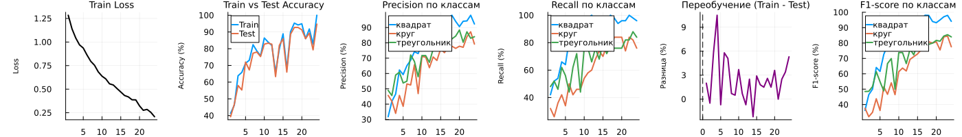
It is interesting to interpret each graph separately. For example, precision grew almost equally for all classes, but the recall score immediately became better for squares, and was always behind for triangles, remaining not the highest by the end of the learning process.
We did not continue training after achieving 100% quality on the test, because there was no point in comparing implementations with each other. But we definitely should have generated more objects for the dataset, since, on average, by the end of training, the model accurately identified squares and circles, but out of the five proposed triangles, on average, one of them "did not notice". Although those that she marked as triangles were indeed triangles (the network showed more "false positive" errors for the "circle" class).
Forecasts from the Julia (Flux) neural network
include("$(@__DIR__)/_scripts/simple_mosaic.jl")
UNKNOWN_DIR = "$(@__DIR__)/unknown";
gr()
plot(create_simple_mosaic(UNKNOWN_DIR, imsize=64))
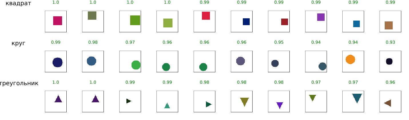
We see pretty good predictions, but this is not so much the result of successful training as the result of long-term work by the designer. The most time-consuming was the selection of the network architecture (number of layers, channels, use of BatchNorm and Dropout) and hyperparameters (learning rate, batch size, augmentation) in order to achieve stable convergence and avoid overfitting on a limited data set. As a result, for example, augmentation was moved to the dataset generating function to simplify the example, as well as due to the fact that this procedure is needed only for triangles.
Export to C and testing
Now we convert the preprocessed images to binary format, generate the C code of the neural network, compile it into an executable file, and visualize the predictions obtained from the C implementation. We knowingly assume that the code will work on platforms where there is no PNG library. Therefore, we convert images to binary format using a separate script. These binary files contain matrices, the elements of which include each color channel of each pixel, represented by a single UInt8 number.
include("$(@__DIR__)/_scripts/convert_png_to_rgb8.jl")
convert_png_to_rgb8("$(@__DIR__)/unknown", "$(@__DIR__)/unknown_rgb8", 64)
Now that we have a dataset with binary images ready, we can download the already trained model and translate it into C code. The key requirement for successful export is full alignment of data formats (RGB8 for images, HWC order of coefficients) and the order of weight traversal between Julia and C, which is achieved by explicit control of indexing and normalization at all stages.
include("$(@__DIR__)/_scripts/generate_cnn_code.jl")

using Flux, BSON
BSON.@load "$(@__DIR__)/model.bson" model classes
model = Flux.testmode!(model)

# Generating the library and the main program
generate_shared_lib(model, 64, length(classes))
generate_main_program(64, length(classes))
We will compile the neural network itself into a library. We also generated the main program, which feeds images from the "unknown_rgb8" folder to the neural network and processes the classification results.
;gcc -shared -fPIC neural_net.c -o libneuralnet.so -lm
;gcc main.c -o classify_unknown -ldl -lm
Interestingly, to run this neural network, we don't need any libraries, either Julia or C. It runs on any system that has a C compiler.
;./classify_unknown
When transferring the model to C, we had to solve several non-trivial tasks: manually implementing convolutions and BatchNorm without third—party libraries, reducing all operations to a single HWC format, accurately reproducing the order of weight traversal (especially critical for multi-channel layers), as well as working with binary image files due to the lack of a PNG library in the target environment - all these The difficulties were successfully overcome.
Forecasts from the neural network in C
include("$(@__DIR__)/_scripts/create_mosaic_from_c_predictions.jl")
run(pipeline(`./classify_unknown`, stdout="pred.txt"))
UNKNOWN_DIR = "$(@__DIR__)/unknown";
gr()
mosaic_grouped = create_mosaic_from_c_predictions("is unknown", "pred.txt", max_images=8)
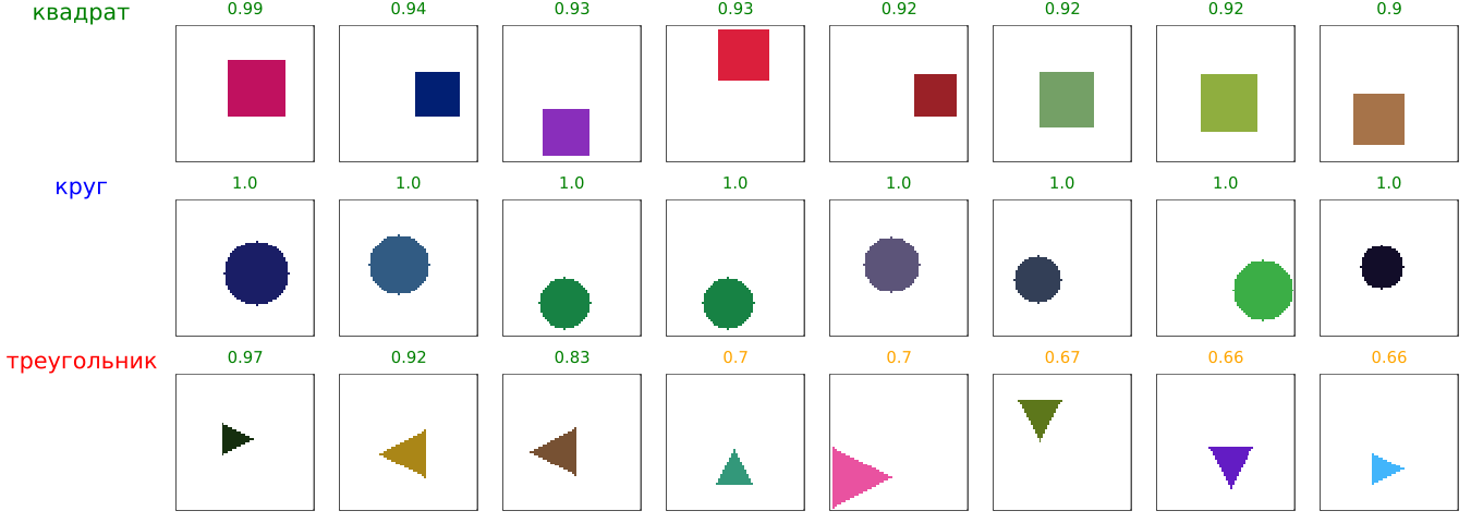
Despite these difficulties, we have demonstrated a full working pipeline, proving that exporting neural networks from Julia to C is possible even with limited resources of the target platform.
include("$(@__DIR__)/_scripts/predict_to_csv.jl")
UNKNOWN_DIR = "$(@__DIR__)/unknown";
predict_to_csv(UNKNOWN_DIR, confidence_threshold=0.4, output_csv="$(@__DIR__)/predictions.csv")
run(pipeline(`./classify_unknown`, stdout="pred.txt"))
include("$(@__DIR__)/_scripts/compare_c_and_julia.jl")
df = compare_c_and_julia()
sort(df)
Conclusion
We have shown how to go through the full cycle of creating a program with a neural network inside: from creating a dataset and training a model on Julia to exporting to C and checking performance, which confirms the fundamental possibility of using the generated code far beyond the Engee engineering platform.