Automatic model assembly and simulation
This example continues the theme of software modeling management, which was previously considered in the community project "Application of software management моделью".
Now let's pay attention to public methods of program management, which allows you to assemble flowcharts (models) from interactive scripts, set the parameters of individual blocks, log outputs, and run a dynamic simulation in a loop with parameter changes.
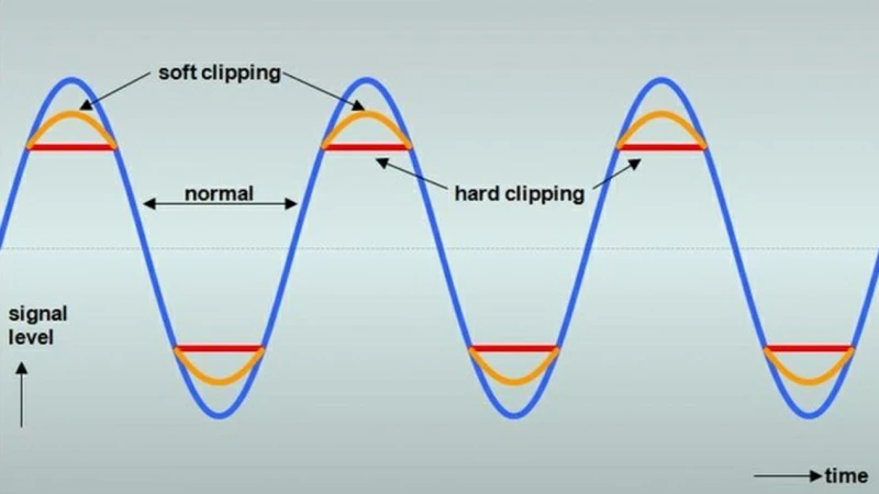
As an example, we will assemble a simplified circuit of a nonlinear power amplifier, and try to consider the distortions of the input sinusoidal signal depending on its level (amplitude). Two nonlinear phenomena will be observed in most standard power amplifiers:
- smooth distortion of the peaks of sinusoidal signals (soft clipping)
- sharp trimming of peaks (saturation, hard clipping)
For the audio signal, this will manifest as "overload" or "distortion".
The blocks that allow you to simulate these phenomena are included in the basic library.
Creating a model
Specify the name of the power amplifier model to be created:
mdlname = "amp_model"
Next, we use the methods create and open to open the model on the canvas:
engee.create(mdlname)
engee.open(mdlname)
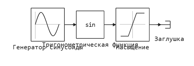
Method add_block this will allow us to add the following blocks of the base library:
- sinusoidal signal source
- trigonometric function block (soft clipping model)
- Saturation block (hard clipping model)
- plug block
engee.add_block("/Basic/Sources/Sine Wave", mdlname*"/")
engee.add_block("/Basic/Math Operations/Trigonometric Function", mdlname*"/")
engee.add_block("/Basic/Discontinuities/Saturation", mdlname*"/")
engee.add_block("/Basic/Sinks/Terminator", mdlname*"/")
Let's connect four blocks in series using the method add-line:
engee.add_line("Генератор синусоиды/1", "Тригонометрическая функция/1")
engee.add_line("Тригонометрическая функция/1", "Насыщение/1")
engee.add_line("Насыщение/1", "Заглушка/1")
And we will automatically arrange the model using the method arrange_system:
engee.arrange_system(mdlname)
As a result, we get a neat and readable flowchart.:
Saving the model to a file with the *.engee extension
engee.save(mdlname * ".engee")
Configuring Block parameters
Method set_param! allows you to specify numerical and string parameters of blocks in the model. We will set the amplitude and frequency of the generated sinusoid, the type of trigonometric function, and the boundaries of the output signal level.
(you can learn more about the settings of the general parameters of the model and simulation from the documentation and the previous example)
engee.set_param!(mdlname*"/Генератор синусоиды", "Amplitude" => 0.75)
engee.set_param!(mdlname*"/Генератор синусоиды", "Frequency" => 2.0)
engee.set_param!(mdlname*"/Тригонометрическая функция", "Operator" => "tanh")
engee.set_param!(mdlname*"/Насыщение", "UpperLimit" => 0.6)
engee.set_param!(mdlname*"/Насыщение", "LowerLimit" => -0.6)
Signal logging and simulation start
First of all, we analyze the outputs of the Sine Wave Generator and the Saturation block using the method set_log:
engee.set_log("Генератор синусоиды/1");
engee.set_log("Насыщение/1");
Let's run the model for dynamic simulation with standard settings using the method run. Let's write the total output of the simulation results to the variable result. Let's select separate variables for the input and output of the nonlinear part of the system, and plot the graph using the function plot:
result = engee.run(mdlname);
x = collect(result["The sine wave generator.1"]);
y = collect(result["Saturation.1"]);
plot(x.time,x.value,lw=2,label="Entrance")
plot!(y.time,y.value,lw=2,label="Exit")
Running the simulation in a loop
We will change the parameters of the signal source block in the loop and run simulations programmatically. The parameters of the amplitude and frequency of the sine wave will vary. The result will be written to the outmatrix variable.:
ampvec = 0.25:0.25:1.25;
n = length(ampvec);
freqvec = LinRange(1,3,n)
outmatrix = zeros(length(x.time),n);
for i = 1:n
    engee.set_param!(mdlname*"/Генератор синусоиды", "Amplitude" => ampvec[i])
    engee.set_param!(mdlname*"/Генератор синусоиды", "Frequency" => freqvec[i])
    tempresult = engee.run(mdlname);
    tempout = collect(tempresult["Saturation.1"]);
    outmatrix[:,i] = tempout.value;
end
We will display the resulting output signals on one axis with the function plot:
plot(x.time,outmatrix,labels=string.(collect(ampvec)'))
And also we will construct the matrix in 3D by the function surface:
surface(collect(freqvec), x.time, outmatrix, c = :rainbow)
Conclusion
In this interactive script, we have reviewed the basic principles of automated model creation and block parameter settings, as well as the possibility of running dynamic simulations in a loop with parameter changes.
engee.close_all()