Time domain flow analysis with EngeeDSP blocks

We continue to get acquainted with the functionality of EngeeDSP using the example of solving a problem that was previously considered in the project. Анализ и обработка во временной области с EngeeDSP.

Main objectives:

visualize the signal
remove the constant component
analyze statistics
smooth the shape

But the task is complicated by the fact that now we are working with a streaming signal, which means that the import of signal samples, analysis and processing must be carried out on the fly. The processing algorithm will only have access to those samples or frames of the signal that arrived at its input at a certain point in the simulation time.

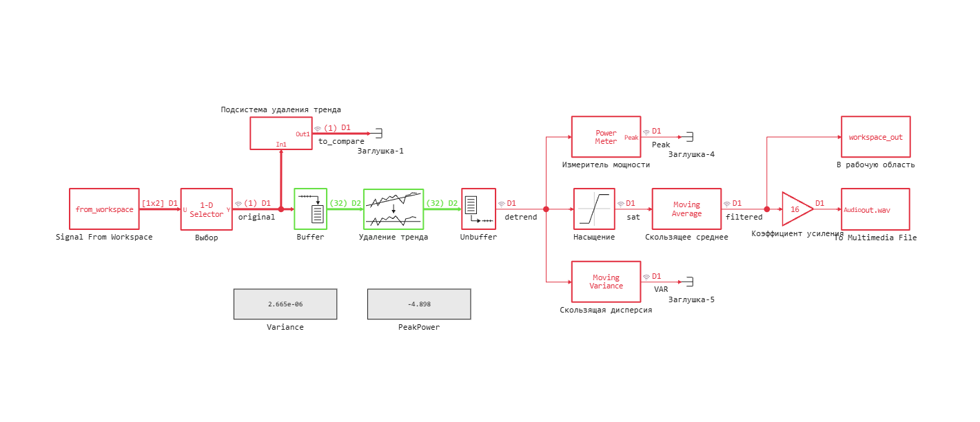
We will consider the model time_analysis_blocks.engee, consisting of specialized blocks of the signal processing library, and we will learn the features of streaming processing in dynamics:

Signal import and visualization

The sensor data is also stored in a text file. data.txt. We read them into the Workspace matrix datamat using the following commands:

# using DelimitedFiles
# datamat = readdlm("data.txt")

The same commands are written in the Callbacks of the model so that the data is automatically loaded into the Workspace when the model is opened.

To read the matrix samples from the Workspace into the model, we use the Signal From Workspace block, and in order to extract the second column from the data matrix, which contains the samples of the signal under study, the block The choice.

Let's run the model on a dynamic simulation and consider the shape of the original signal. original.

mdlname = "time_analysis_blocks.engee";
engee.open(mdlname);
engee.run();

We can observe the original signal in time in the Visualization window:

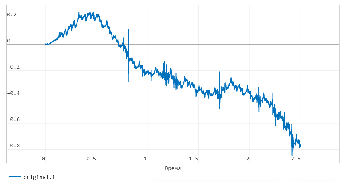
The signal contains a constant component, which it would be useful for us to get rid of for further analysis and processing.

Removing the permanent component

When working in the script, the entire signal was available to us from the first to the last sample, and the constant component was removed by approximating its shape with a 12th-order polynomial, but in the case of streaming processing, we need to use a different approach.

The model compares two ways to remove a "trend" on small signal frames.

First, using the Trend Removal block, which approximates successive segments of the signal with a first-order polynomial (i.e., a line). Before this operation, the scalar signal is buffered into vectors of 32 samples without overlap.

In addition, the signal passes through a subsystem, inside which the "trend" is calculated as the average value in a window of 64 samples, and it is subtracted from the delayed signal.:

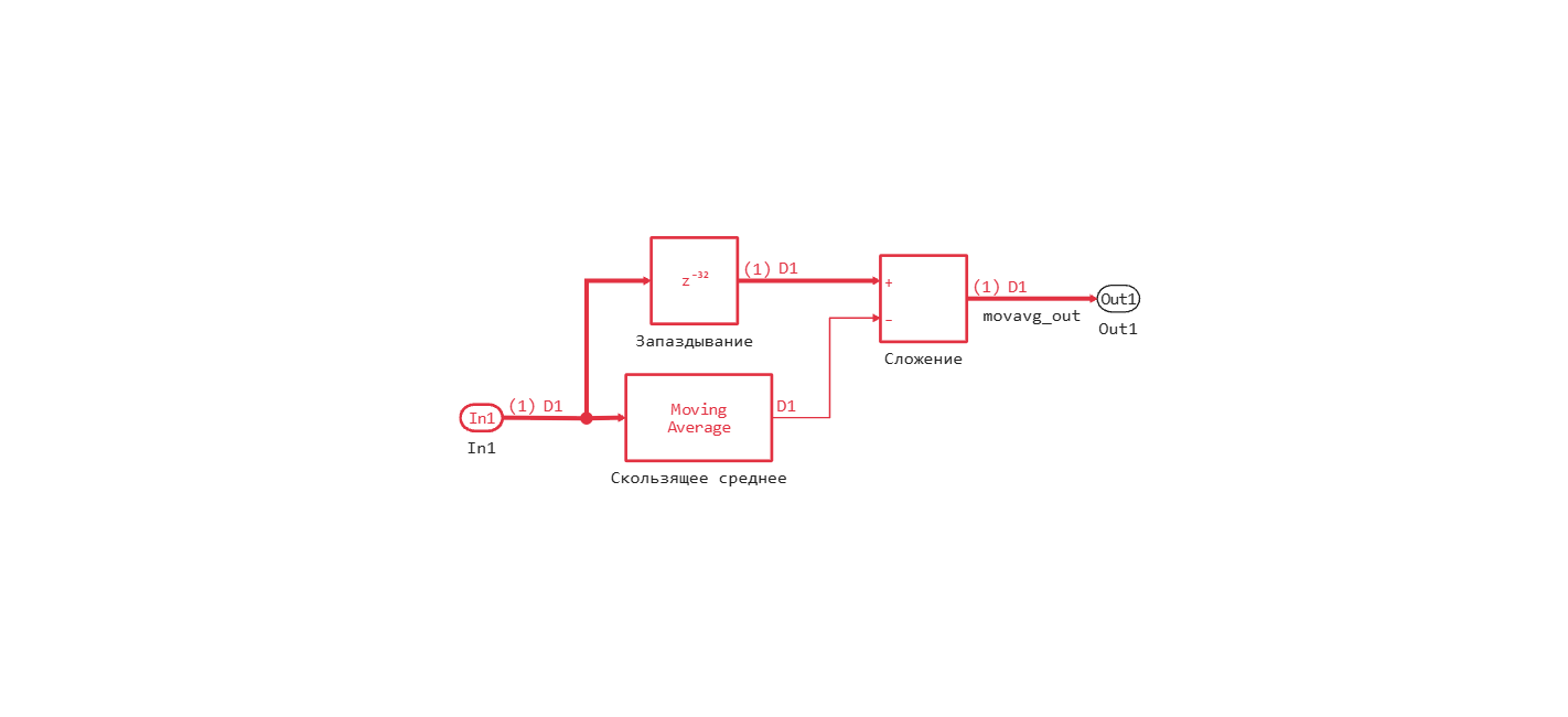
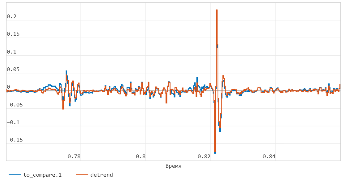
By comparing the output signals of these two operations in the Visualization window, you can make sure that the approaches work approximately the same - you just need to adjust the size of the window (or frame) correctly. The signal will go further along the processing chain detrend from the output of the Unbuffer block:

Signal Statistics

To calculate statistics, the signal Processing library has many blocks for both vector and "sliding" statistics calculations.

The model calculates signal parameters such as peak power and variance. The results are recorded in the log and also displayed on the Display blocks ** during the dynamic simulation. Consider the graph of variance over time:

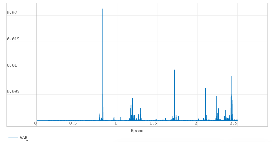
It can be noted that the dispersion graph clearly shows peaks corresponding to local extremes of the signal without a constant component.

Smoothing the waveform

With streaming processing, we are again faced with a situation where the values of the entire signal are not available to us, and we cannot use an analog of the function. findpeaks. Using statistics and user logic, it is realistic to find local extremes within the frame under consideration, but this is computationally expensive, and for this model it is sufficient to perform the operation of threshold limiting emissions using the Saturation block.

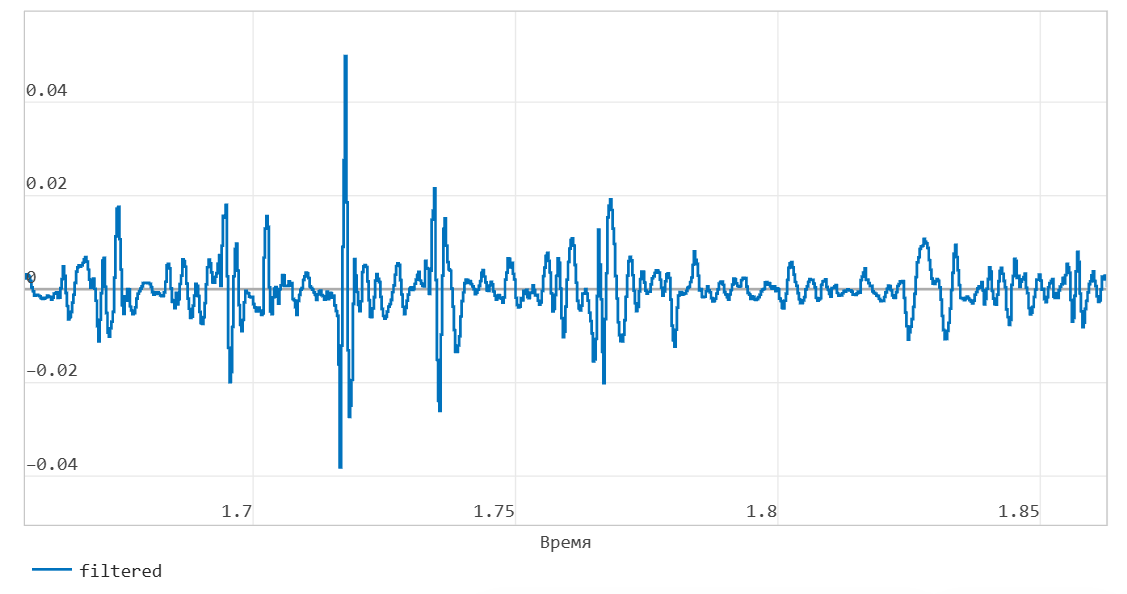
The final filtering will be performed using the Moving Average block on a small window of 4 counts. The resulting waveform after processing:

Uploading simulation results

To record the signal in the variable area, we use the block In the workspace. We will also record the signal as a *.wav file so that you can listen to it in any media player.

DF = collect(workspace_out);
time = DF.time;
value = DF.value;
plot(time,value,leg=false,xguide = "Time, from")

Conclusion

We got acquainted with the functionality of the EngeeDSP blocks (signal Processing library) for tasks of streaming visualization, analysis and processing in time, and also compared approaches to solving a similar problem in the Engee script from this примера.