Custom Incandescent lamp model
The purpose of the material is to show the full path from the physical formulation of the problem to the user component in the Engee physical modeling language and its verification in an alternating current circuit.
There is already a separate section in the [Engee Community] with examples of custom physical компонентов](https://engee.com/community/ru/catalogs/projects?page=1&meta-query;={"state"%3A{"published"%3A{}}%2C"modeling_in_engee"%3A{"physical_one_d_modeling"%3A{"custom_components"%3A{}}}}). We continue this topic and analyze the lamp model, the resistance of which increases when the filament is heated.
The Engee physical modeling language is declarative: the developer records the relationships between physical quantities and differential equations, and the causality and numerical solution are determined by the solver. The syntax and purpose of the constructions are given in the official documentation.
Mathematical model
The filament is considered as an electrical resistance with thermal inertia. When turned on, the thread is cold, so its resistance is low. As the lamp heats up, its resistance increases, and the current decreases to its nominal value.
The switching resistance and the nominal resistance are determined by the set voltage and currents.:
The linear temperature dependence of the resistance is given by the expression
Electrical power It is spent on heating the filament at the moment of switching on and transferring heat to the environment.:
where – the coefficient of heat transfer, and – thermal time constant. From the established nominal regime, we obtain
In the model C. Initial value corresponds to an unheated thread.
How the component works @engeemodel
Any custom physical component starts with a design @engeemodel Имя begin ... end. Specialized sections of the type are placed inside it. @... begin ... end.
@iconbinds a component to a fileicon.svg, which sets its appearance on the canvas.@nodesannounces two non-directional electrical portspandnlikeEngeePhysicalFoundation.Electrical.Pin. In the electrical domain, the port contains a potentialvand the stream variablei. Metadataviewthe signatures and the sides of the port placement are set.@parametersIt contains values that can be adjusted before simulation. After the comma, the metadata is written in square brackets: the unit of measurement and the description of the parameter.@variablesintroduces continuous unknownsdelta_T,iandv. Their values are determined by the entire system of equations, not by the sequential execution of lines. Initial valuedelta_T = 0.0and high priority helps to set an unheated initial state.@intermediatesIntermediate equations are set, which are calculated directly from the parameters and variables. Resistances, heat transfer coefficient, and power components are included here.@branchesconnects the internal currentiwith streaming port variables: writei:(p.i, n.i)sets the direction of the branch and ensures the balance of currents when connecting components.@equationscontains a physical relationship. Tilda~denotes equality in the system of equations, andder(delta_T)– the derivative of temperature with respect to time.
The official examples in the documentation show the port type without parentheses. The file code is shown below /user/custom_lamp/lamp.ngpc.
Full component code
The full contents of the file are shown below. lamp.ngpc.
# Description of an incandescent lamp in the Engee physical modeling language
# The model simulates an increase in resistance when heated. When turned on, you can see a large inrush current. The initial state is that the lamp is not warmed up.

@engeemodel Lamp begin

    @icon begin
        "icon.svg"
    end

    #Announcement of electrical ports
    @nodes begin
        p = EngeePhysicalFoundation.Electrical.Pin(), [view = ("+", "left")]
        n = EngeePhysicalFoundation.Electrical.Pin(), [view = ("-", "right")]
    end

    #declaring parameters
    @parameters begin
        V_nom = 220.0, [unit = "V", description = "Rated voltage"]
I_inrush = 5.0, [unit = "A", description = "Cold lamp starting current"]
I_nom = 0.413, [unit = "A", description = "Heated lamp rated current"]
alpha = 0.004, [unit = "1/K", description = "Temperature coefficient of resistance"]
time_coefficient = 0.025, [unit = "s", description = "Thermal time constant"]
end

    #declaration of unknown variables
    @variables begin
        delta_T = 0.0, [unit = "K", description = "Temperature change of the filament relative to the initial state", priority = "high", access = Private] #potential variable
        i = 0.0, [unit = "A", description = "Current", access = Private]        #streaming variable
        v = 0.0, [unit = "V", description = "Voltage", access = Private] #potential variable
    end

    #declaration of intermediate variables that are calculated explicitly from parameters and variables
    @intermediates begin
        R_cold = V_nom / I_inrush, [unit = "Ohm"]                           #Cold lamp resistance through inrush current and rated voltage
        R_nom = V_nom / I_nom, [unit = "Ohm"]                               #Lamp resistance in operating mode through rated current and rated voltage
        k = alpha * I_nom^2 * R_nom / (R_nom / R_cold - 1), [unit = "W/K"]  #heat transfer coefficient from the heat balance equation with zero derivative (UR)
R = R_cold * (1 + alpha * delta_T), [unit = "Ohm"]                  #Resistance in transition mode
        P_electrical = i^2 * R, [unit = "W"]                                #Electrical power
        P_loss = k * delta_T, [unit = "W"]                                  #Heat output
        P_heat = time_coefficient* k * der(delta_T), [unit = "W"]           #Lamp heating power
    end

    #current flow rule
    @branches begin
        i:(p.i, n.i) #stream variable
    end

    #Lamp equations
    @equations begin
        v~ p.v - n.v #voltage is a potential difference
        v ~ R * i #Ohm's law
        time_coefficient * k * der(delta_T) ~ i^2 * R - k * delta_T #heat balance equation
end

end
The verification scheme
The component is connected in series with an AC voltage source of 220 V of the current value and a frequency of 50 Hz. The switch closes at 0.04 s. An ammeter, a voltmeter, and RMS units allow simultaneous observation of instantaneous and effective voltage and current values. The Solver Configuration block is required for the physical network, and the electrical grounding sets the reference potential.
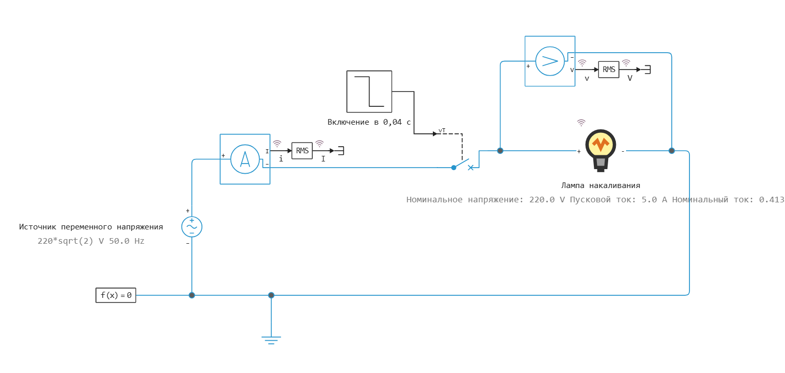
Figure 2 is a test circuit of a lamp with an alternating voltage source.
Simulation results: voltage and current
Up to 0.04 s, the key is open, so the lamp voltage and current are zero. After the short circuit, the instantaneous voltage has an amplitude of about B, and the current value is 220 V. The stepped section of the RMS curve is related to the fact that the meter needs to accumulate data for the calculation window.
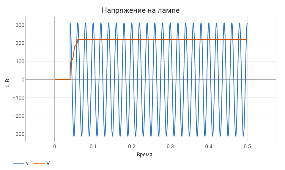
Figure 3 – Instantaneous and effective voltage across the lamp.
Immediately after switching on, the cold resistance is 44 ohms. Therefore, when switched on near the amplitude of the sine wave, the instantaneous current reaches approximately A, which is consistent with the peak in Figure 4 and the set effective value of the inrush current As
it warms up, the resistance increases, the current amplitude decreases, and the effective value tends to the nominal current value set in the parameters of 0.413 A. The sign of the instantaneous current changes with the polarity of the source; negative values do not mean reverse heating, since the heat balance uses .
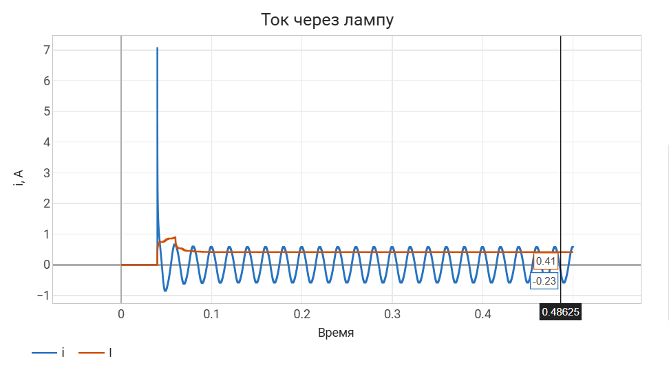
Figure 4 – Starting process and steady-state lamp current.
Simulation results: resistance
Before switching on, the resistance retains a cold value of 44 ohms. After the voltage is applied, it increases rapidly and reaches the nominal resistance range. Ohms. Small ripples of steady-state resistance occur because the instantaneous power with a sinusoidal current, it pulsates with twice the mains frequency, that is, about 100 Hz. The thermal time constant smooths out these pulsations, but in the accepted concentrated model it does not eliminate them completely.
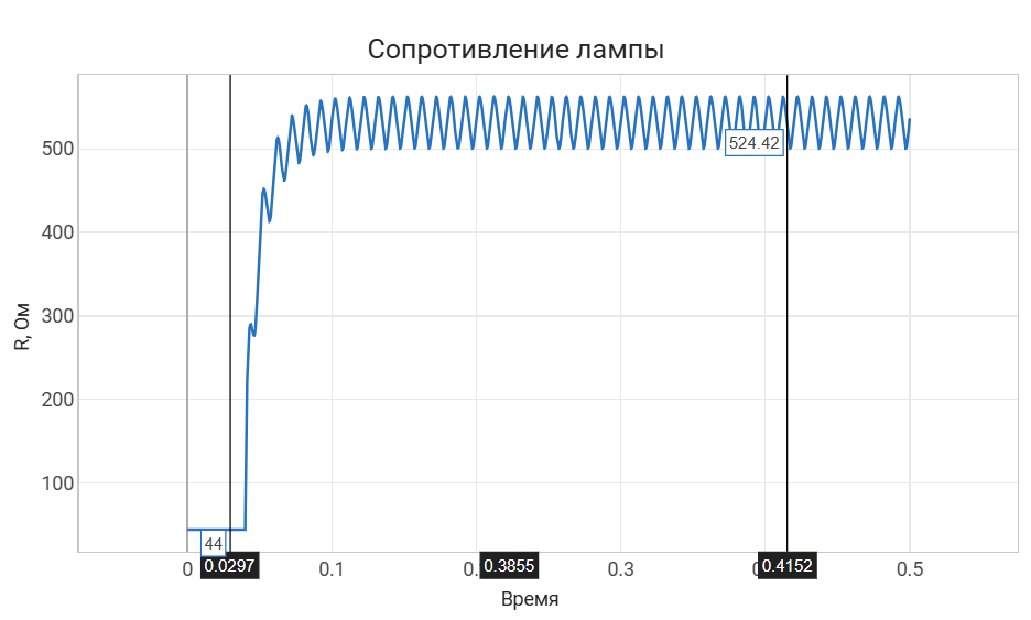
Figure 5 – Increase in thread resistance during heating.
The graphs are consistent with each other: an increase in resistance is accompanied by a decrease in the inrush current, while the effective source voltage remains 220 V. The model reproduces the main qualitative property of an incandescent lamp – a large cold thread current and its limitation after warming up.
Used sources
- Engee Physical Modeling Language – the purpose of the declarative language and the structure of the documentation section.