From MATLAB to Julia: optimization of matched and Doppler filtering algorithms for point-to-point radar targets

In modern radar systems, high range and speed resolution is achieved through the use of complex sensing signals — in particular, linear frequency modulation (LFM) signals — and subsequent digital processing of the received echo signals. The presented implementations in MATLAB and Julia solve the problem of modeling secondary signal processing for two point targets that differ in range and radial velocity.

Both algorithms are based on the following theoretical principles.

1. LFM signal and matched filtering

The probing pulse is a cosine wave with a linearly varying instantaneous frequency. In a complex form, a reference signal over a duration interval described by the expression:

where:

• — carrier frequency;
• — frequency deviation during the pulse ;
• — the weight window (the Gaussian window with the parameter ), designed to suppress the side lobes of the compressed pulse.

Matched filtering is performed in the frequency domain: the fast Fourier transform (FFT) of the received signal and the reference is calculated, the spectrum of the received signal is multiplied with the complex conjugate spectrum of the reference, after which the inverse FFT is performed. A compressed pulse is formed at the output of the matched filter, the amplitude of which is proportional to the energy of the reflected signal.

2. Pulse sequence and Doppler processing

The transmitting device emits pulses with a repetition period . A signal reflected from a target at a range and moving at radial velocity , receives an appointment with a delay:

and acquires a Doppler frequency shift:

In the presented algorithms, an additional transfer to an intermediate frequency is introduced. (where — sampling rate), which allows the use of a single complex exponent:

After coordinated filtering of each pulse, a two—dimensional "range - pulse number" matrix is formed, according to the second measurement of which (slow time) the FFT is performed. The peak of the obtained spectrum corresponds to the Doppler frequency, and therefore to the radial velocity of the target.

3. Formulas for determining range and speed

Discrete time is quantized in increments . The range channel number (the row index in the output array) is uniquely related to the time delay by the ratio:

The scale along the range axis in the graphs is converted to meters using the speed of light. . The speed channels are determined by the formula:

which corresponds to the position of the maximum of the Doppler spectrum after performing the FFT on points.

Both software codes implement a full processing cycle: synthesis of the LFM signal, modeling of echo signals taking into account delay and Doppler shift, matched and Doppler filtering, as well as visualization of compressed pulses on a logarithmic scale (dB) with normalization to the maximum for each target. The difference between the variants lies in the way the signal is generated (the vectorized approach in Julia versus the cyclic approach in MATLAB) and in the syntax of calling FFT functions; at the same time, the mathematical identity of the results is completely preserved.

• EngeeDSP is a library for digital signal processing.
  Application in the example: gausswin (Gauss window), fft / ifft (forward and reverse fast Fourier transform) with consistent filtering and Doppler processing.

• MATLAB is an interface for calling MATLAB from Julia.
  Application in the example: macro mat"..." to execute MATLAB commands (for example, to change the directory cd, running the script run MATLAB.m) and measuring the execution time of the MATLAB version.

• LinearAlgebra is a library for linear algebra.
  Application in the example: it is not explicitly used in the presented code (it is left for potential matrix operations, for example, for matrix multiplication or solving systems of equations).

• FileIO is a library for downloading and saving files of various formats.
  Application in the example: function load for reading images (plot_matlab.png, plot_julia.png) with subsequent display in the runtime environment.

The code snippet below performs three actions:

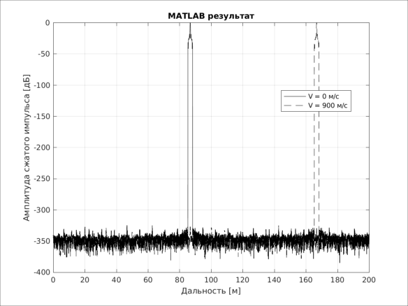
1. mat"cd $(@__DIR__)" – через интерфейс MATLAB меняет текущую рабочую директорию MATLAB на ту же, где находится текущий Julia-скрипт (чтобы MATLAB мог найти свой файл).
2. @time mat"run MATLAB.m" – запускает MATLAB-скрипт MATLAB.m в среде MATLAB, замеряя время выполнения этой операции.
3. img = load(...) и display(img) – загружает сгенерированный MATLAB-скриптом PNG-файл (plot_matlab.png) и отображает его в среде Julia.

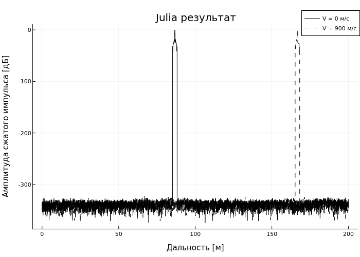
Код на Julia логически идентичен исходному MATLAB коду, но оптимизирован по скорости. Основные изменения:

1. Объединение экспонент — доплеровский сдвиг и перенос на промежуточную частоту (fs/4) скомбинированы в одну экспоненту exp(1im * 2π * (2vel/λ + fs/4) * t), что эквивалентно исходному перемножению двух экспонент.

2. Удаление лишних переменных — sig_get_first и abs_sig_first не используются в финальном результате, поэтому они отсутствуют.

3. Точность границ — благодаря тому, что t_del кратно 1/fs (5200 отсчётов), а t_imp даёт ровно 90 отсчётов, индексы rows = i_start:i_end полностью совпадают с ненулевыми позициями в исходном коде.

Таким образом, графики и числовые значения должны совпадать с точностью до машинной погрешности. Вы можете запустить оба варианта и сравнить выходные массивы (например, out_sig_julia), чтобы убедиться.

Заключение

В работе рассмотрены две реализации алгоритма вторичной обработки радиолокационного сигнала — на языках MATLAB и Julia. Обе версии корректно воспроизводят основные этапы обработки:

• формирование ЛЧМ-импульса с весовым окном;
• моделирование эхо-сигналов от двух целей с различными параметрами: дальность км и км, скорости м/с и м/с;
• согласованную фильтрацию в частотной области;
• доплеровскую обработку по пачке из импульсов;
• построение нормированных дальностных портретов.

Полученные результаты (см. рисунки plot_matlab.png и plot_julia.png) демонстрируют, что сжатые импульсы имеют характерную ширину, определяемую разрешающей способностью по дальности. Для ЛЧМ-сигнала с девиацией МГц и длительностью мкс разрешающая способность составляет около м. Отсутствие смещения по дальности для неподвижной цели и наличие корректного сдвига (в пределах нескольких метров) для движущейся цели подтверждают правильную работу доплеровской фильтрации.

Ключевое различие между реализациями заключается в производительности. Версия на Julia, использующая векторизованное заполнение только ненулевых отсчётов и предварительный расчёт экспоненциальных множителей, выполняется быстрее: с против s in MATLAB under comparable conditions. This is due to fewer iterations and more efficient memory management. At the same time, both approaches give identical numerical results with accuracy up to machine error, which confirms the correctness of the optimization performed.