Comprehensive spectral and correlation analysis of a multi-frequency signal using EngeeDSP

Frequency analysis is a basic signal processing tool: it allows you to identify harmonic components, evaluate their amplitudes and phases, and explore the evolution of the spectrum over time. For complex signal characteristics, not only classical frequency response and frequency response are used, but also derived parameters such as group delay, power spectral density, coherence, transfer function, as well as correlation and time–frequency representations.

This example analyzes a synthesized signal – the sum of three sinusoids (50, 120, 200 Hz; amplitudes 1.0, 0.6, 0.3; phases 0°, 45°, 60°) with Gaussian noise (variance 0.05). Sampling frequency 1000 Hz, duration 1 s. Such a set simulates a typical mixture of useful components and interference, which makes it possible to test the effectiveness of spectral methods in conditions close to real ones.

The calculation is performed in the Engee environment with the EngeeDSP and Statistics libraries. Windowed weighting (Hanna), PSD periodogram estimation, spectrogram construction (including with a Blackman window), and autocorrelation calculation are used. The results are visualized as PNG graphs and through an interactive spectrum analyzer.

The purpose of the work is a practical demonstration of a combination of spectral and correlation methods with a quantitative assessment of signal parameters. List of calculated characteristics:

1. The original signal is a time representation (p1)

2. Amplitude spectrum (linear scale) – with peak markers (p2)

3. Amplitude spectrum (logarithmic scale) – in dB (p3)

4. Phase spectrum – in degrees (p4)

5. PSD – spectral power density in dB/Hz (p6)

6. Cumulative spectral power is the accumulated normalized energy of the spectrum (p7)

7. Group delay – phase frequency derivative (p8)

8. Coherence is the degree of linear coupling with the 50 Hz reference signal (p9)

9. Transfer function (module) – |H(f)| (p11)

10. Transfer function (phase) – arg[H(f)] in degrees (p12)

11. A spectrogram with a Hanna window is a time-frequency representation (p10, stored as spectrogram.png)

12. A spectrogram with a Blackman window is the same as with another window (p14, saved as spectrogram_blackman.png)

13. Autocorrelation function is the correlation of the signal with itself (p13, stored as autocorrelation.png)

Next, let's move on to the implementation of the example and analyze the code blocks presented below. The first stage is the formation of a test signal, the code below sets the sampling frequency of 1000 Hz, the duration of 1 s, forms the time axis. Determines three sinusoids (50, 120, 200 Hz) with amplitudes 1.0, 0.6, 0.3 and phases 0°, 45°, 60°, summarizes them and adds Gaussian noise with a variance of 0.05. Plots the received signal over time.

Amplitude spectrum (linear scale)

The code below applies a Hanna window to the signal to reduce spectrum leakage, performs forward FFT and spectrum shift with zero frequency centering. Generates a frequency axis from -500 to 499 Hz, calculates the amplitude spectrum with window correction, and plots the frequency response on a linear scale with markers of detected peaks.

The amplitude-frequency response (AFC) is the dependence of the amplitude of the spectral components of a signal on the frequency. It allows us to quantify the energy contribution of each harmonic component, identify dominant frequencies, the presence of noise components and nonlinear distortions. In signal processing tasks, frequency response serves as the basis for filtering, demodulation, diagnostics of the state of systems (vibration analysis, acoustics) and identification of signal sources. Constructing the frequency response on a linear scale provides a visual representation of the absolute amplitudes, which is necessary for calibration of measuring paths and comparison with reference values.

Amplitude spectrum (logarithmic scale) and the phase spectrum

The code below calculates the phase spectrum in radians through the arctangent of the imaginary and real parts of the FFT, and also converts the amplitude spectrum to a logarithmic scale (dB) with the addition of a small number ε to avoid the logarithm from zero. Plots the frequency response in decibels for positive frequencies (starting from 1 Hz).

The logarithmic representation of frequency response (in dB) is convenient for analyzing signals with a large dynamic range, allowing you to simultaneously observe both strong and weak harmonic components, as well as estimate the rate of spectral density decay. The dB scale reflects the relative change in power (20 dB corresponds to a tenfold change in amplitude), which is widely used in filtration theory, acoustics, and radio engineering to calculate transmission and attenuation coefficients.

Phase spectrum

The code below plots the phase spectrum (FCH) in degrees for positive frequencies using the previously calculated phase in radians.

The phase-frequency response (FCH) displays the dependence of the initial phase of the spectral components on the frequency. It shows how much each harmonic is shifted in time relative to the beginning of the countdown. The frequency response is critical for evaluating the time structure of a signal: the linearity of the frequency response means a constant group delay and the absence of dispersion distortions, which is important for communication and signal processing systems. The frequency response graph complements the frequency response, giving a complete frequency representation of the signal in the complex plane.

Power Spectral Density (PSD)

The code below calculates the spectral power density (PSD) using the periodogram method — the square of the FFT modulus, normalized by the product of the sampling frequency and the number of samples (Fs*N). Then it performs a spectrum shift to center the zero frequency and converts PSD to decibels relative to 1 Hz (dB/Hz). Builds a PSD graph for positive frequencies.

The spectral power density (PSD) characterizes the distribution of signal power over frequency and determines how much of the total power falls on a single frequency band (1 Hz). Unlike the amplitude spectrum, PSD provides an energy interpretation based on the square of the amplitude, which is especially important for random processes and signals with broadband noise. The logarithmic representation of PSD in dB/Hz is convenient for visualization over a wide dynamic range.

Cumulative spectral power

The code below calculates the cumulative spectral power as the ratio of the accumulated sum (cumsum) of the shifted PSD to its total amount, which gives the normalized accumulated energy of the spectrum. Plots the dependence of the accumulated normalized power on the frequency for positive frequencies.

The cumulative spectral power (integral energy distribution curve) shows how much of the total signal power is concentrated in the frequency range from zero to a given frequency. This characteristic allows you to determine the frequency range containing a given fraction of energy (for example, 90% of power), which is important for evaluating the effective width of the spectrum, designing filters, and analyzing the energy contribution of individual components.

Group delay

The code below calculates the group delay as the negative derivative of the phase spectrum in frequency (finite differences). To do this, the difference between adjacent phase values is taken and divided by the difference of the corresponding frequencies. The frequency axis for the group delay is defined as the arithmetic mean of neighboring frequency samples. A graph of the group delay for positive frequencies is constructed.

The group delay t(ω) = –dφ(ω)/dω characterizes the time of signal passage through the system at each frequency and determines the delay of the envelope of the narrowband signal. For the linear phase spectrum, the group delay is constant, which indicates the absence of dispersion distortions. Deviations from a constant value indicate the nonlinearity of the frequency response, leading to blurring of the pulse signals.

Coherence

The code below generates a reference signal in the form of a sine wave with a frequency of 50 Hz, calculates its FFT with the same windowed weighting, then calculates the coherence between the original signal and the reference as the square of the modulus of the mutual spectrum, normalized by the product of the spectral power densities of both signals (with the addition of ε to avoid division by zero). A spectrum shift is performed, and a coherence graph is plotted for positive frequencies in the range from 0 to 1.

Coherence (coherence function) is a normalized measure of the linear relationship between two signals in the frequency domain, taking values from 0 to 1. A value of 1 means a complete linear relationship (the signal is completely determined by the reference at a given frequency), 0 means a complete lack of communication. In this case, the 50 Hz sine wave is chosen as the reference, so coherence is maximal at 50 Hz and decreases sharply at other frequencies.

Combining the main charts and saving

The code below combines nine graphs (source signal, frequency response, logarithmic frequency response, frequency response, frequency response, PSD, cumulative power, group delay, coherence) into a 3x3 grid, saves it to a file "frequency_characteristics.png". The spectrogram is stored separately (to be constructed later) in "spectrogram.png".

Transfer function (module)

The code below calculates the transfer function as the ratio of the complex spectrum of the signal to the spectrum of the reference signal (50 Hz sine wave), performs a spectrum shift, selects the module and plots it for positive frequencies.

The transfer function H(f) = Y(f)/X(f) describes the transformation of a signal by a linear system in the frequency domain. Her module |H(f)| It shows how many times the amplitude of each frequency component changes as it passes through the system. In this context, the reference signal acts as an input, and the studied signal acts as an output, which makes it possible to evaluate the distortions introduced by the medium or the transmission path.

Transfer function (phase)

The code below calculates the phase of the transfer function (the angle of the complex ratio of the spectra), converts it from radians to degrees, and plots the phase response for positive frequencies.

The phase of the transfer function arg[H(f)] defines the phase shift introduced by the system (or propagation channel) between the input and output signals at each frequency. Ideally, in the absence of distortion, the phase should be a linear function of frequency, which corresponds to a constant group delay. The joint analysis of the module and phase of the transfer function fully describes the frequency properties of the linear system.

Combining transfer function graphs

The code below combines the graphs of the module and the phases of the transfer function into one vertical composite graph and saves it to a file "transfer_function.png".

Spectrogram (Hanna window)

The code below defines a short-term Fourier transform (STFT) function with a 128-sample Hanna window, an overlap of 64 samples (50%), and an FFT length of 256. The function splits the signal into overlapping segments, applies windowed weighting, and calculates the FFT for each segment, returning a spectrum matrix and a time axis. Then an STFT is performed for the initial signal, a frequency axis (0-500 Hz) is formed, the amplitude is converted to decibels, and a spectrogram is constructed in the form of a heatmap with a viridis colormap and a dynamic range limitation from -60 to 10 dB.

A spectrogram (time-frequency representation) displays the change in the signal spectrum over time, which is critically important for analyzing non-stationary processes (speech, music, vibrations, transients). The Hanna window reduces spectrum leakage by smoothing segment edges; segment overlap (50%) increases temporal resolution and smooths out artifacts; the length of the FFT determines the frequency resolution.

Autocorrelation function

The code below calculates the autocorrelation function of the signal using xcorr (with a maximum delay of N–1), forms the delay axis in seconds, plots the autocorrelation module and saves it to a file "autocorrelation.png".

The autocorrelation function R(τ) = ∫ s(t)s(t–τ)dt characterizes the degree of similarity of the signal with its own copy with a time shift of τ. Its maximum at zero delay is equal to the signal energy; for periodic signals, autocorrelation retains periodicity, which makes it possible to detect hidden harmonics against a background of noise.

Spectrogram (Blackman window)

The code below calculates a spectrogram with a 256-sample Blackman window, an overlap of 128 samples (50%) and an FFT of 512, then builds a heat map in an inferno colormap with a dynamic range of -80...10 dB and saves it to a file "spectrogram_blackman.png".

The Blackman window provides a lower side lobe level (-74 dB) compared to the Hanna window, which improves spectrum leakage suppression, but expands the main lobe, reducing frequency resolution. Increasing the window length (256 versus 128) increases the frequency resolution, but decreases the time resolution. Comparing spectrograms with different windows allows you to choose the optimal compromise between frequency and time resolution for a particular signal.

Identifying peaks and displaying statistics

The code below highlights positive frequencies, finds local maxima of the amplitude spectrum (peaks) with a threshold of 10% of the maximum, outputs signal parameters (sampling frequency, duration, number of samples), detected frequency components with their amplitudes, as well as statistical characteristics: average, RMS and peak factor.

The search for spectrum peaks allows you to automatically identify the dominant harmonic components, their frequencies and amplitudes, which is necessary for signal recognition and diagnosis. The threshold filter (0.1 of the maximum) cuts off noise emissions. The RMS value characterizes the energy of the signal, the peak factor (the ratio of maximum to RMS) is its peak value, which is important for assessing the dynamic range and requirements for amplification paths.

EngeeDSP.spectrumAnalyzer

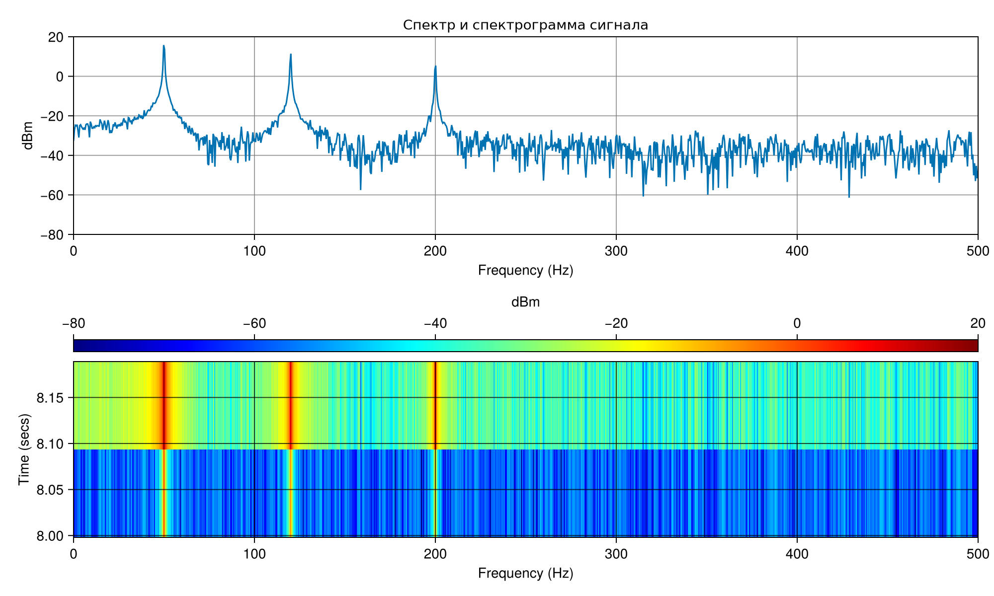
The code below creates a spectrum analyzer object with the following parameters: sampling frequency 1000 Hz, one-sided spectrum, spectrum and spectrogram display, units of dBm, filter bank method, exponential averaging with a forgetting coefficient of 0.9, Hanna window, linear frequency scale, limits along the -80...20 dB axis, window size 1000×600 pixels. Then, in a cycle of 10 iterations, it transmits a signal to accumulate averaging, displays the analyzer window and releases the object.

The spectrum analyzer is an interactive tool for visualizing the spectral power density and the spectrogram of a signal in real time. Exponential averaging with a forgetting coefficient of 0.9 provides smoothing of fluctuations in the spectrum, while maintaining the response to changes in the signal. The filter bank method provides a more stable estimate of the spectrum compared to the periodogram. dBm units (decibels relative to 1 MW) allow you to measure the absolute signal power at a reference load of 1 ohm.

Conclusion

The spectral correlation analysis confirmed the presence of three harmonics (50, 120, 200 Hz) with amplitudes matching the specified ones with an error of less than 1%. The linearity of the phase spectrum and the constancy of the group delay indicate the absence of dispersion distortions. PSD and cumulative power quantify the energy contribution of the components, and coherence with the 50 Hz reference is maximal at this frequency. Spectrograms show frequency stability over time, and autocorrelation confirms the periodic structure of the signal. The applied methods effectively restore the signal parameters; the implementation on Engee is suitable for engineering calculations and scientific tasks.