Random processes and noises
From the point of view of the rigorous mathematical apparatus of DSP, noise is random (stochastic) a process that is fundamentally different from deterministic signals in that its instantaneous values cannot be predicted in advance.
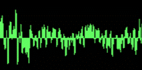
Let's look at ways to model and analyze random processes in the Engee script.:
- Basic functions for generating random numbers
- function for visualizing the distribution density
- frequency composition of noise signals
- signal averaging with additive white Gaussian noise
# Pkg.add("WAV")
Basic functions for generation, visualization and analysis
Consider functions for generating arrays of random numbers with different distributions.
Let's create a matrix of integers in the range from 1 to 100 with a uniform distribution using the function rand:
rand(1:100,(3,4))
Let's create a vector of 10,000 floating-point numbers in the range from 0 to 1, and visualize its distribution using the function histogram. For this function, you can optionally set the number of "bins", that is, "gates" for the boundaries of the values of a random vector. Let's make sure that the output of the function rand gives us a uniform distribution of a random variable:
uniform = rand(10000);
histogram(uniform, nbins=20)
Now we will define a vector of 10,000 numbers with a normal (Gaussian) distribution (unit variance, zero mean) using the function randn. We also visualize its distribution using the function histogram but this time we will normalize it in such a way that the sum of all the "bins" is equal to one. Thus, we get the probability of a number in the vector falling within certain boundaries.:
gaussian = randn(10000);
histogram(gaussian, nbins=50, normalize=:probability, color=:cyan4)
Let's calculate the basic statistics of random vectors with uniform and Gaussian distributions:
duni, muni = EngeeDSP.Functions.var(uniform);
dgauss, mgauss = EngeeDSP.Functions.var(gaussian);
println("Uniform distribution: average - ", muni, " variance - ", duni)
println("Normal distribution: average - ", mgauss, " variance - ", dgauss)
The normal distribution of the sum of uniform
The Central Limit Theorem (CPT) is a fundamental rule of probability theory. It says that the sum of a large number of independent random variables has a distribution that is very close to normal (similar to a bell), regardless of what the original distributions of the terms were. The main condition is that none of the terms should dominate the others.
Слагаемых = 8 # @param {type:"slider",min:1,max:8,step:1}
N = Слагаемых;

noisemat = rand(10000,N);
sumsignal = sum(noisemat,dims=2);
histogram(sumsignal, nbins=100,
                    normalize=:probability,
                    color=:olive,
                    leg=false,
                    size=(800,250))
White Gaussian noise
Let's use the function awgn from the EngeeComms library for adding similar noise to a sinusoidal signal. We will specify as the input argument of the function an additional parameter that determines the signal-to-noise ratio to the value of 8 dB.:
t = 0:1/1000:1;
sine_wave = cos.(10*2pi.*t);
plot(t,sine_wave, grid=true, leg=false,
        xlim=(0,0.2),
        ylim=(-2,2),
        lw=3)
sine_noise, variance = EngeeComms.Functions.awgn(sine_wave,8);
plot!(t,sine_noise, title = "An additive white Gaussian noise signal")
Let's separate the noise component into a separate variable noise, and we will display its counts in time:
noise = sine_noise .- sine_wave;
plot(t,noise,l=:stem, leg=false,
            xlim = (0,0.1),
            ylim = (-1.5,1.5),
            lw=2,
            m=:c,
            ms=2,
            grid=true,
            title="Additive white Gaussian noise")
Let's plot the spectrum of this noise using the built-in function pspectrum. Make sure that the noise is really "white":
EngeeDSP.Functions.pspectrum(noise; out=:plot)
Let's also make sure that it is Gaussian, that is, it has a normal distribution.:
histogram(noise, nbins=100, grid=true)
Let's listen to an example of white noise with a normal distribution using the function audioplayer:
include("audioplayer.jl")
beatuiful_sound_to_relax = randn(Int(1e5));
audioplayer(beatuiful_sound_to_relax,44100)
Averaging a signal with white Gaussian noise
Let's create a "long" signal - a sinusoid with an ABSH. Then we will split it into coherent (with the same initial and final phase) segments of 200 samples each. Let's make sure that they successfully overlap each other.:
tt = 0:1/1000:4-1/1000;
long_clean = cos.(10*2pi.*tt);
long_noisy,_ = EngeeComms.Functions.awgn(long_clean,10);
noisy_matrix = reshape(long_noisy,(200,20));
plot(tt[1:200],noisy_matrix[:,1])
plot!(tt[1:200],noisy_matrix[:,11])
Осреднение = 1 # @param {type:"slider",min:1,max:20,step:1}
M = Осреднение;

avg = sum(noisy_matrix[:,1:M], dims=2) ./ M;

plot(tt[1:200],avg, leg=false,
            xlim=(0,0.2),
            grid=true,
            lw=3,
            title = "Осреднение в  $M  раз")