Parameterization of SDM based on measurements
This example shows how to determine the parameters of a permanent magnet synchronous motor based on experimental measurements.
In order to determine the parameters of the SDPM engine, we will conduct three experiments. The desired values of the engine parameters are known to us in advance, and we will compare them with the values obtained from the experiments.
Data from the engine documentation:
nPolespairs = 2;        # Number of pairs of poles
iRated = 2.5;           # Current at rated speed and load (A)
rpmRated = 7500;        # Rated speed (rpm)
torqueRated = 0.07;     # Torque at rated speed (NM)

torqueStall = 0.28;     # Preset torque (NM)
iStall = 8.5;           # Peak current (A)

inertia = 5e-6;                        # Moment of inertia (kg·m2)
viscousDamping = 1.13e-6;              # Coefficient of viscous friction
staticFriction = 7e-4;                 # Coefficient of dry friction
coulombFriction = 0.8*staticFriction;  # Coulomb friction coefficient

R = 3.43;               # Resistance (Ohms)
L = 0.53e-3;            # Inductance (Gn)

# Parameters of the PMSM block
torqueConstant = 2/3*torqueStall/iStall; # Torque Constant (Nm/A)
emfConstant = torqueConstant; # Constant counter-EMF (V*s/rad)
PM = torqueConstant/nPolespairs; # Permanent Magnet Flow Coupling (Vb)

# Controller parameters and flags
rpmDemand = rpmRated; # Preset speed (rpm)
enableDrive = 1; # Enabling control
dt = 1e-4; # Sampling period of the controller (s)
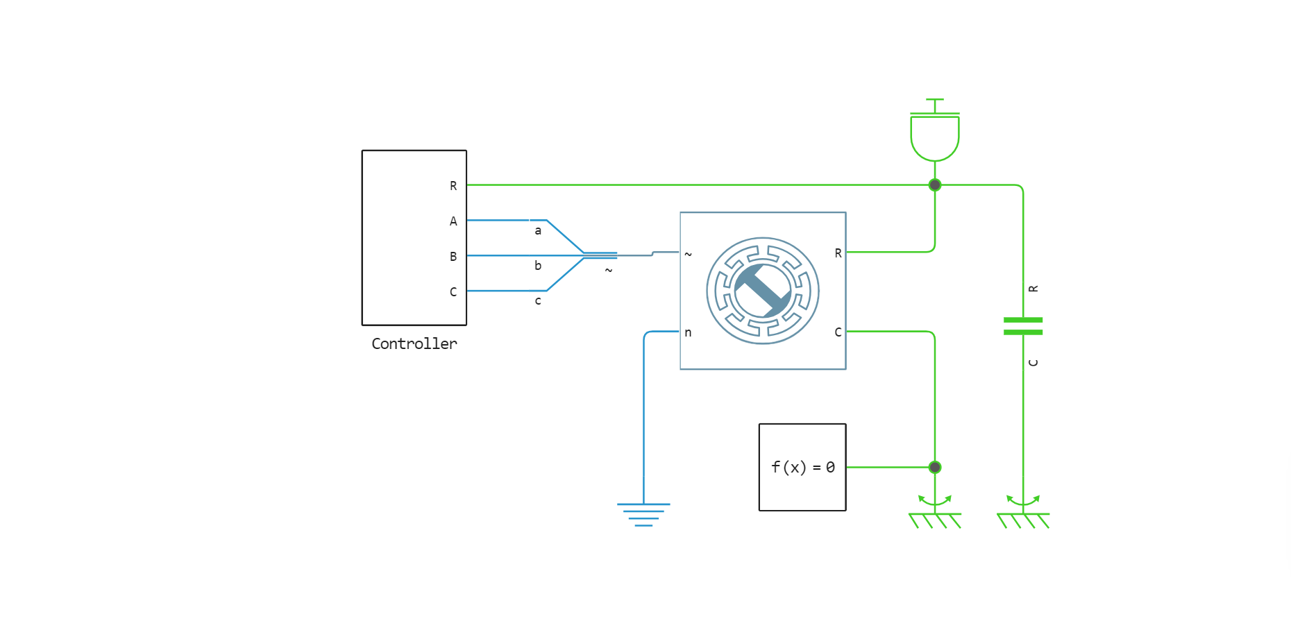
Test 1. Determination of R and L with a stationary rotor
The first experiment is carried out on an engine with a locked rotor. A voltage step is applied between the phases and the transient response process is studied. The resulting time constant τ is determined by the values of the resistance and inductance of the stator:
Let's set the initial rotation angle of the rotor:
rotorangle = -90/(nPolespairs);
Launching the model:
engee.addpath(@__DIR__)

if "PMSMFromMeasurement1" in [m.name for m in engee.get_all_models()]
    m = engee.open( "PMSMFromMeasurement1" ) # loading the model
else
    m = engee.load( "PMSMFromMeasurement1.engee" )
end
results1 = engee.run(m, verbose=true)
Reading data from a model:
t = results1["uab"].time;       # Time
uab_1 = results1["uab"].value;  # Voltage between phases A and B
ia  = results1["ia"].value;     # Current in phase A
Calculate the resistance from the values of steady-state voltage and current.
The windings a and b are connected in series in the experiment, so we divide the resulting resistance by 2:
R_e = uab_1[end] / ia[end] / 2;
Let's find the time constant of the circuit - this is the time it takes for the current to reach the value from the established:
idx = findfirst(x -> x >= (0.63 * ia[end]), ia);
tau = t[idx];
From the formula let's express and calculate the inductance L:
L_e = R_e * tau;
The expected transition process:
iEstimated = uab_1[end] / (2 * R_e) * (1 .- exp.(-t .* R_e ./ L_e));
In the graph below, you can compare the measured current from the model and the current graph obtained from the calculations.
using Plots
plotlyjs();
plot(t, ia, xlabel="Time, c", ylabel="Current, A", w = 2, label="Measured current", linecolor =:blue)
plot!(t, iEstimated, xlabel="Time, c", ylabel="Current, A", w = 2, label="Expected current", linecolor =:green)
plot!([tau, tau], [0, ia[end]], linecolor =:red, line =:dashdot, label="τ" )
xlims!(0, 10*tau)   # Setting x-axis limits
ylims!(0, ia[end])  # Setting the limits of the y-axis

annotate!(0.0008, 4.5, text(string("R is the reference = ", R, " Om"), :left, 10))
annotate!(0.0008, 4, text(string("R measured = ", round(R_e, digits=2), " Om"), :left, 10))
annotate!(0.0008, 3.5, text(string("L Reference = ", L*1000, " mGn"), :left, 10))
annotate!(0.0008, 3, text(string("L Measured = ", round(L_e*1000, digits=2), " mGn"), :left, 10))
annotate!(tau, 1, text(string("The measured time constant = ", round(1000*tau, digits=3), " ms"), :left, 10))
Test 2. Determination of the constant counter-EMF
In the second experiment, the motor rotates without electrical load. This allows us to estimate the constant counter-EMF.
Note that the counter-EMF constant, expressed in SI units, is equal to the torque constant of the motor, so only one constant is calculated in this example.
.png)
Launching the model:
if "PMSMFromMeasurement2" in [m.name for m in engee.get_all_models()]
    m = engee.open( "PMSMFromMeasurement2" ) # loading the model
else
    m = engee.load( "PMSMFromMeasurement2.engee" )
end
results2 = engee.run(m, verbose=true)
Reading data from a model:
t = results2["uab"].time;       # Time
uab_2  = results2["uab"].value; # Voltage A-b
Determination of the counter-EMF constant
The counter-EMF constant it can be calculated using the formula:
where – voltage drop in phase a of the motor,
– angular velocity of the motor shaft.
The torque constant is equal to the counter-EMF constant expressed in SI units.
wRef = rpmRated*2*pi/60;        # Angular velocity of the rotor (rad/s)
vPeakLL = maximum(abs.(uab_2)); # Peak line voltage (V)
vPeakLN = vPeakLL/sqrt(3);      # Peak voltage phase-neutral (V)
emfConstantE = vPeakLN/wRef;    # wq counter-EMF constants
The graph below shows the counter-EMF that occurs when the experimental engine is moving at rated speed.
The number of pole pairs can be determined by calculating the number of periods of current change per rotation of the rotor.
plot(t, uab_2, xlabel="Time, c", ylabel="Counter-EMF", label="Counter-EMF of the experimental engine", w = 2)
annotate!(0.0013, -20, text(string("Counter-EMF reference constant = ", round(emfConstant,digits=4), " In*s/rad"), :left, 10))
annotate!(0.0013, -25, text(string("Counter-EMF measured constant = ", round(emfConstantE,digits=4), " In*s/rad"), :left, 10))
3. Determination of coefficients of friction and moment of inertia
In the third experiment, the unloaded motor is controlled by a controller.
In a previous experiment, a constant of the moment was obtained. With its help, by converting the stator currents, the friction coefficients can be calculated.
.png)
Variables required for controller simulation:
rpm2rad = 2*pi/60;
rad2rpm = 60/(2*pi);
powermax = torqueRated*rpmRated*2*pi/60;
Kp = 0.01;
Ki = 2.0;
ts = 0.0001;
t2eq_Iq = 2/(3*nPolespairs*PM);
Let's measure the mechanical torque required to maintain a constant rotational speed at four different speeds.
The torque required at lower speeds is primarily aimed at overcoming dry friction, at higher speeds - viscous friction.
The graph shows the measured moments for the four speeds. A straight line is drawn through these points. The zero-velocity intersection gives the dry friction coefficient, and the slope gives the viscous friction coefficient.
function trapz(x, y)
    n = length(x)
    integral = 0.0
    for i in 1:n-1
        integral += (x[i+1] - x[i]) * (y[i+1] + y[i]) / 2
    end
    return integral
end
rpmVec = [0.25, 0.5, 0.75, 1.0]*rpmRated;
trqVec = zeros(size(rpmVec));
for i=1:length(rpmVec)
    if "PMSMFromMeasurement3" in [m.name for m in engee.get_all_models()]
        m = engee.open( "PMSMFromMeasurement3" ) # loading the model
    else
        m = engee.load( "PMSMFromMeasurement3.engee" )
    end
    rpmDemand = rpmVec[i];
    engee.set_param!("PMSMFromMeasurement3", "StopTime" => 2*60/rpmDemand)
    results3 = engee.run(m, verbose=true)
    t = results3["ia"].time;        # Time from the model
    ia_3  = results3["ia"].value;   # phase current-a from the model
    idx = findfirst(x -> x >= (60/rpmDemand), t);
    temp = trapz(t[idx:end],(ia_3[idx:end]).^2)
    iaRms = sqrt(temp/(t[end]-t[idx]));
    trqVec[i] = 3*torqueConstant*iaRms;
end
rpmDemand = rpmRated;
scatter(rpmVec, 1000*trqVec, title="Mechanical torque losses", xlabel="Speed, m/s", ylabel="Moment, mN*m", w = 2, label="Measured values", legend=:bottomright )
using Polynomials
coef = coeffs(fit(2*pi/60*rpmVec, trqVec,1));
estimatedStaticFriction = coef[1];
estimatedViscousDamping = coef[2];
rpmVec0 = [0; rpmVec];
plot!(rpmVec0, 1000*(estimatedStaticFriction.+rpmVec0*2*pi/60*estimatedViscousDamping), label="Linear approximation")
annotate!(trqVec[end], 2.1, text(string("Dry friction coefficient reference = ", staticFriction), :left, 10))
annotate!(trqVec[end], 2.0, text(string("Dry friction coefficient measured = ", round(estimatedStaticFriction,digits=6)), :left, 10))
annotate!(trqVec[end], 1.9, text(string("The coefficient of viscous friction is the reference = ", viscousDamping), :left, 10))
annotate!(trqVec[end], 1.8, text(string("Coefficient of viscous friction measured = ", round(estimatedViscousDamping, digits=9)), :left, 10))
The second graph shows an engine deceleration test. For this test, the required torque is set to zero or the motor is switched off.
Using the measured deceleration, at the specified values of the friction and damping moments, it is possible to determine the moment of inertia of the motor rotor.
enableDrive = 0;
engee.set_param!("PMSMFromMeasurement3", "StopTime" => 2*60/rpmDemand)
if "PMSMFromMeasurement3" in [m.name for m in engee.get_all_models()]
    m = engee.open( "PMSMFromMeasurement3" ) # loading the model
else
    m = engee.load( "PMSMFromMeasurement3.engee" )
end
results4 = engee.run(m, verbose=true)
enableDrive = 1;
t = results4["rpm"].time;       # Time from the model
rpm  = results4["rpm"].value;   # rotor speed
plot(t, rpm, xlabel="Time, c", ylabel="Speed (rpm)", label="The deceleration test", w = 2)
initialTorque = -staticFriction - rpmRated*2*pi/60*viscousDamping;
initialAccel = 2*pi/60*(rpm[end]-rpm[1])/(2*60/rpmDemand);
estimatedInertia = initialTorque/initialAccel;
annotate!(0, 7465, text(string("The moment of inertia is the reference = ", inertia, " kg×m^2"), :left, 10))
annotate!(0, 7460, text(string("Moment of inertia measured = ", round(estimatedInertia,digits=6), " kg×m^2"), :left, 10))
Conclusion
In this example, we have determined the parameters of a permanent magnet synchronous motor based on experimental measurements.
To do this, we conducted three tests. In the first test, we found the resistance and inductance of the motor winding, in the second we determined the counter-EMF constant, and in the third we determined the coefficients of friction and moment of inertia.
The values found experimentally are comparable to the engine parameters from the documentation.