Determination of liquid pressure at different tank heights
In this example, we will demonstrate one property of a thermally conductive liquid, due to which the temperature may vary slightly at different heights when it is in the tank.
Description of the model
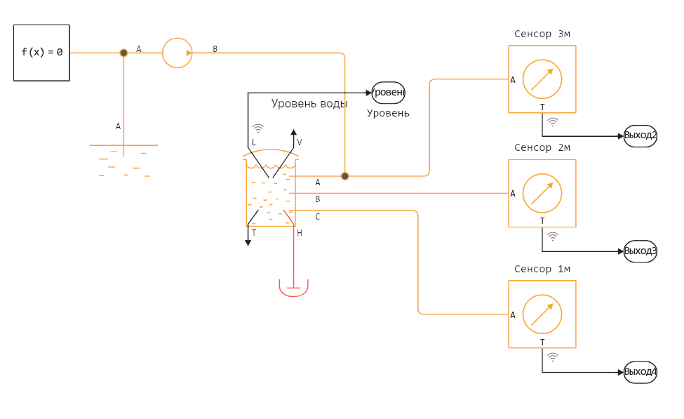
Let's create a system consisting of a tank, a pump that pumps liquid from the tank into it, and several sensors.
In a real liquid described by the equation of state, the temperature at different heights will vary slightly due to changes in pressure in the liquid column (hydrostatic effect) and the thermodynamic properties of the medium. Let's examine this issue strictly.
For a liquid obeying the equation of state, the distribution of temperature and pressure is determined by the hydrostatic law , equations of state and and several additional effects (thermal equilibrium, compression/expansion). Here - pressure, - temperature, - height, - density, - acceleration of free fall, - specific internal energy.
The lower layers of the liquid are under slightly higher pressure, so the liquid at the bottom of the tank will be slightly warmer than on the surface.
In reality, many other thermal effects are unlikely to allow the experiment to be observed in the formulation presented here. Mixing, the heat effect of the pump, and heat transfer through the tank walls can all have an effect on the temperature of the liquid.
Running the model and analyzing the results
In our model, the tank has a diameter of 1 , liquid flows into it, pumped by a pump at a speed of 1 kg / s, the calculation is carried out from 0 to 1000 seconds. The liquid temperature sensors are located at heights of 1, 2 and 3 m.
model_name = "tank_temperature_at_different_heights";
model_name in [m.name for m in engee.get_all_models()] ? engee.open(model_name) : engee.load( "$(@__DIR__)/$(model_name).engee");
res = engee.run( model_name );
During the observation, the liquid level in the tank rose by 1m. Let's see how the temperature readings changed at different heights.
gr()
using Plots.PlotMeasures

plot(
    plot( res["Water level"].time, res["Water level"].value, label=false, title="Water level, m",
      xlabel="Time, from", ylabel="Height, m" ),
    plot( res["The sensor is 2 m.1"].time,
      [res["The sensor is 1m.1"].value res["The sensor is 2 m.1"].value res["The sensor is 3 m.1"].value],
      label=["1m" "2nd floor" "3m"], title="Temperature sensors", xlabel="Time, from", ylabel="Temperature, K"),
    size=(1000,400), titlefont=font(11), guidefont=font(10), left_margin = [10mm 0mm], bottom_margin = 30px
)
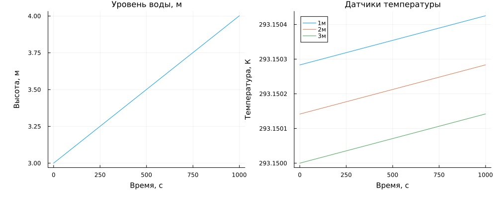
Between 1m and 2m, the sensors show different temperature values, but the scale of the difference can hardly be changed in reality – for 1m, the temperature drops by 1.41e-4 К (ten thousandths of a degree). But we can see that the temperature at the bottom of the tank is slightly higher than at the surface.
res["The sensor is 2 m.1"].value[1] - res["The sensor is 1m.1"].value[1]
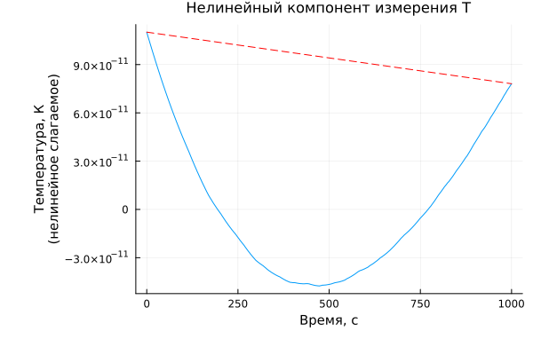
If you take one of the graphs from the temperature sensor and subtract the linear trend, you can even see a very small non-linearity.:
t = res["The sensor is 1m.1"].time
v = res["The sensor is 1m.1"].value
a = [t.^0 t.^1] \ v

difference = v.- (a[1] .+ a[2].*t)

plot( t, difference, label=false )
plot!( [t[1],t[end]], [difference[1],difference[end]], ls=:dash, c=:red, label=false )
plot!(title = "The nonlinear component of the T measurement", xlabel="Time, from", ylabel="Temperature, K\n(nonlinear term)",
    titlefont=font(11), guidefont=font(10), left_margin = [10mm 0mm], bottom_margin = 30px)
Conclusion
Using a simple example, we have shown how a virtual experiment formulated using blocks from the thermally conductive liquid library allows us to demonstrate some theoretical effects that are quite difficult to observe empirically in educational laboratory settings. But they will manifest themselves in more complex cases, and these are effects that can be dangerous to neglect.