Step-down transformer
Introduction
This example demonstrates the operation of a step-down single-phase transformer.
Description of the model
The example model uses blocks from the fundamental section of the Engee library for physical modeling. The transformer is designed for power , the operating frequency , input voltage and a day off. It is assumed that the efficiency is equal to , the no-load magnetization current is and leakage reactivity - . Core losses are not taken into account. It is assumed that the dependency the core material is linear.
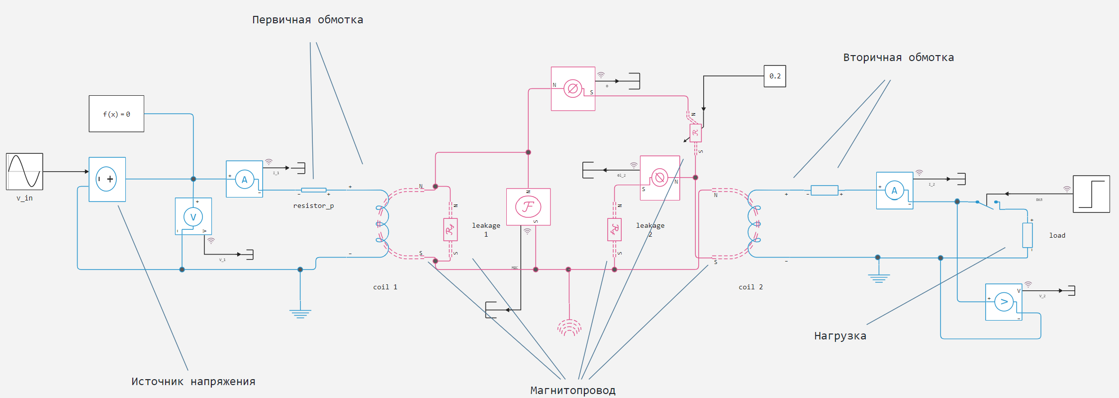
Initially, the transformer is idling. At a moment in time the rated load "load" is switched on. Due to the resistance of the winding and the inductance of the dissipation, the voltage of the secondary winding drops from before . A current is generated on the secondary winding of the transformer .
Simulation
Let's download and execute the developed model.
Example path = @(__DIR__);
Имя_модели = "electrical_transformer";
Путь_модели = joinpath(Путь_примера, Имя_модели*".engee")

if the model name is ∉ getfield.(engee.get_all_models(), :name)
    engee.load(Model path);
end

model = engee.run(Model name);
We will get the variables displayed in the model for further construction.
# Time
t = модель["V_1"].time;
# Voltage
V_1 = модель["V_1"].value;
V_2 = модель["V_2"].value;
# Currents
I_1 = модель["I_1"].value;
I_2 = модель["I_2"].value;
# Magnetic fluxes and MDS
Ф = модель["F"].value;
Ф2σ = модель["Fl_2"].value;
F = модель["MDS"].value;
Simulation results
We will plot graphs of electrical variables - voltages and currents of the primary and secondary windings.
# Connecting the Plots library and the backend
using Plots
plotlyjs()

plot(t, [V_1 V_2]; layout = (2,1), subplot = 1, ylabel = "Voltage, V", label = ["V_1" "V_2"], title="Voltages and currents")
plot!(t, [I_1 I_2]; subplot = 2, ylabel = "Current, A", label = ["I_1" "I_2"], xlabel = "Time, c")
As can be seen from the voltage and current graphs, the transformer lowers the voltage and increases the current. After connecting the rated load secondary winding to the circuit, rated currents begin to flow through the windings.
Let's plot the magnetic variables - the main magnetic flux. , magnetic flux leakage through the secondary winding and magnetomotive force (mds).
plot(t, Ф.*1e3; layout = (3,1), subplot = 1, ylabel = "Stream, MB", label = "F", title="Magnetic variables")
plot!(t, Ф2σ.*1e6; subplot = 2, ylabel = "Flow, mcVb", label = "F2σ", color=:green)
plot!(t, F; subplot = 3, ylabel = "MDS, And⋅in", label = "MDS", color=:red, xlabel = "Time, c")
As can be seen from the graphs, the main magnetic flux after connecting to the secondary load transformer decreases by the magnitude of the leakage magnetic fluxes, and a magnetomotive force is formed in the magnetic circuit.
Conclusion
In this example, a 220/12 V step-down transformer operating at rated load is considered. The dynamics of the electric and magnetic variables of the system was considered.