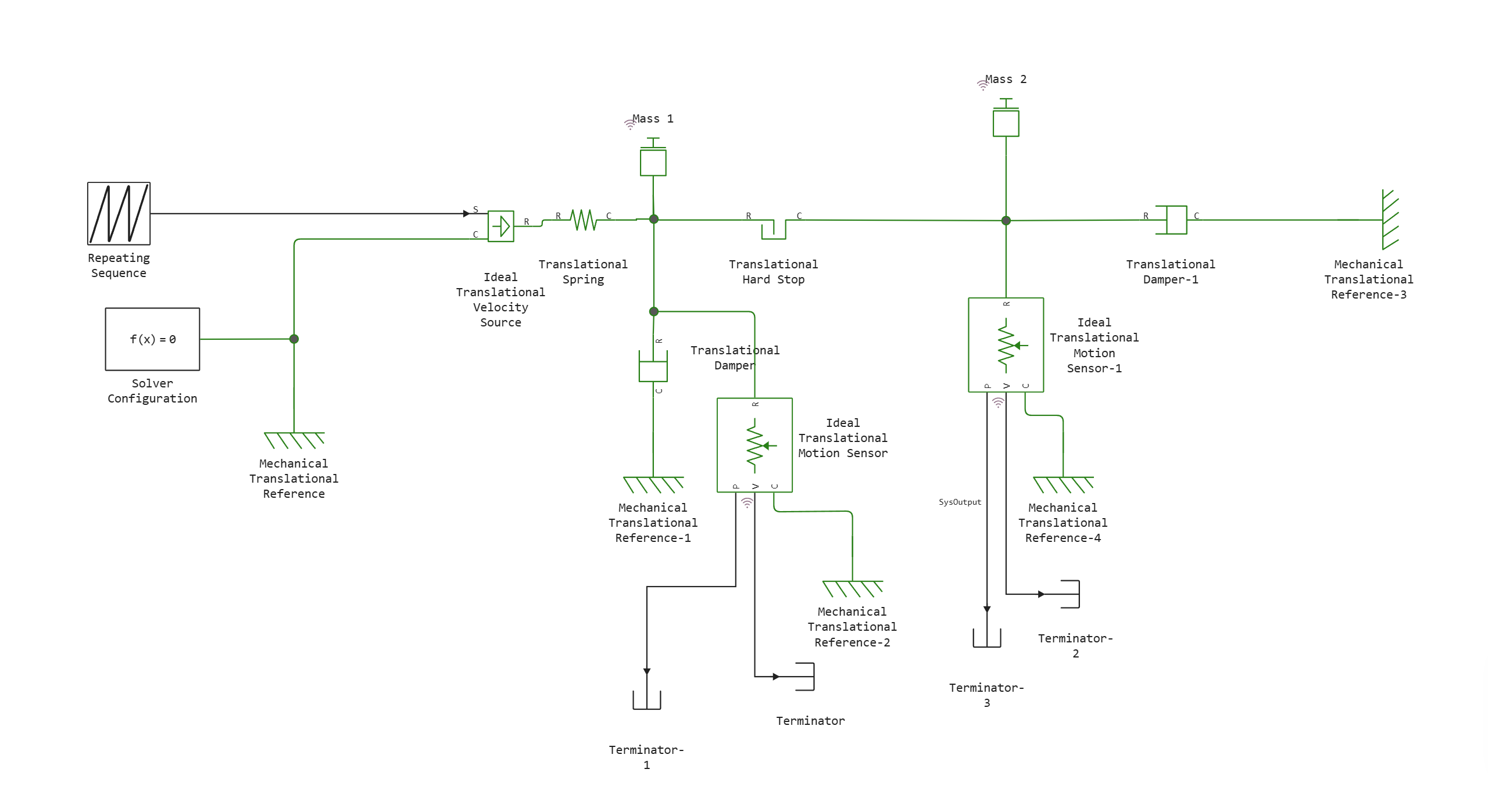
Mechanical system with rigid limiter of translational motion
This example shows two masses connected by a rigid limiter. Mass 1 is driven by an ideal source of velocity. When the direction of the input velocity changes, Mass 2 does not move until Mass 1 reaches the other end of the gap modeled by a translational rigid limiter.
Model diagram:
Defining the function to load and run the model:
In [ ]:
function start_model_engee()
    try
        engee.close("mechanical_system_translational_hardstop", force=true) # closing the model
        catch err # if there is no model to close and engee.close() is not executed, it will be loaded after catch.
            m = engee.load("$(@__DIR__)/mechanical_system_translational_hardstop.engee") # loading the model
        end;

    try
        engee.run(m) # launching the model
        catch err # if the model is not loaded and engee.run() is not executed, the bottom two lines after catch will be executed.
            m = engee.load("$(@__DIR__)/mechanical_system_translational_hardstop.engee") # loading the model
            engee.run(m) # launching the model
        end
end
Out[0]:
Launching the model:
In [ ]:
try
    start_model_engee() # running the simulation using the special function implemented above
    catch err
    end;
Output of simulation results from the simout variable:
In [ ]:
res = collect(simout)
Out[0]:
Writing results to variables:
In [ ]:
P1 = collect(res[7]); # Mass transfer 1 "mechanical_system_translational_hardstop/Ideal Translational Motion Sensor.2")
P2 = collect(res[5]); # Moving mass 2 ("mechanical_system_translational_hardstop/SysOutput")
v1 = collect(res[8]); # Mass velocity 1
v2 = collect(res[3]); # Mass velocity 2
Simulation results:
In [ ]:
using Plots
plot(P1[:,1], P1[:,2], linewidth=3, xlabel= "Time, from", ylabel= "Displacement, m", legend=:bottomright, label="Weight 1")
plot!(P2[:,1], P2[:,2], linewidth=3, label="Weight 2")
Out[0]:
In [ ]:
using Plots
plot(v1[:,1], v1[:,2], linewidth=3, xlabel= "Time, from", ylabel= "Speed, m/s", legend=:bottomright, label="Weight 1")
plot!(v2[:,1], v2[:,2], linewidth=3, label="Weight 2")
Out[0]: