Simulation of an arc steelmaking furnace in static mode
In this example, static modeling and analysis of current and voltage harmonics for a DSP-100NZA arc steelmaking furnace with a capacity of 100 tons and a transformer capacity of 50 MVA are considered.
Introduction
The arc steelmaking furnace (chipboard) is a key unit of modern metallurgy, where the high-temperature electric arc that occurs between the electrodes and the metal charge serves as the main source of energy for remelting scrap metal into high-quality steel. The widespread use of chipboard, especially in the production of steel from scrap, is due to their cost-effectiveness and environmental friendliness, and the prospects of the technology are inextricably linked to further efficiency gains and reduced impacts on the energy system. However, the chipboard is an extremely difficult object to analyze and control due to its pronounced nonlinearity, stochastic arc discharge, and dynamic changes in electrical parameters during melting. It is this complexity that makes it critically important to conduct an in-depth study of adequate chipboard replacement schemes, which are the basis for analyzing operating modes, designing and optimizing control systems. The development of effective electrode control systems is necessary to stabilize arc power, minimize flicker, and increase energy efficiency. In parallel, a thorough analysis of the harmonic composition of the consumed current and voltage on the furnace tires is of paramount importance, since the chipboard is a powerful source of higher harmonics that cause distortion of the voltage curve in the supply network, equipment overload and potential electromagnetic compatibility problems. The study of these aspects is necessary to ensure reliable operation of the furnace itself, reduce network losses and comply with electricity quality standards.
Mathematical description
There are several approaches to the mathematical description of the elements of an electrical chipboard replacement circuit. One such approach, describing the nonlinearity of the resistance of an electric arc, is given in [1]. We'll take him as an example.
The description of the arc resistance given in the article:
Let's present it as directional blocks in the subsystem "Arc resistance calculation".
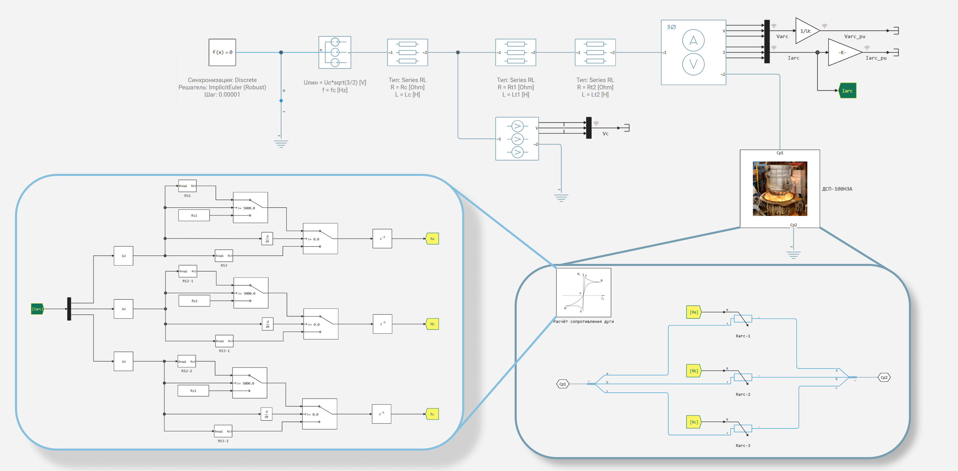
The Engee model
The example model - electric_arc_furnace.engee.
The electrical circuit includes:
-
consecutive RL-цепочки cable line, primary and secondary windings of furnace transformer,
-
phase sensor напряжения for measuring the voltage on the primary winding,
-
current and voltage sensor for measuring current and voltage in DSP phases,
-
linear variable resistors in each phase to simulate arc resistance,
-
Auxiliary elements: grounding нейтрали , neutral порт and splitter фаз.
In the model, the following signals are written to the simout variable:
-
Vc- three-phase voltage at the input of the furnace transformer [V], -
Varc- voltage at each phase of the chipboard [V], -
Varc_pu- relative voltage at each phase of the chipboard [O.E.], -
Iarc- current in each phase of the chipboard [A], -
Iarc_pu- relative current in each phase of the chipboard [O.E.],
The model parameters are also set according to the data from the publication, their definition is given below.:
Uc = sqrt(2)*573  # Amplitude phase voltage of the network (V)
fc = 50.0         # Network frequency (Hz)
Rc = 0.0528e-3; Xc = 0.468e-3; Lc = Xc/(2pi*50)  # Cable Parameters: R(Ohms), X(Ohms), L(Ohms)
Rt1 = 0.05e-3; Xt1 = 0.35e-3; Lt1 = Xt1/(2pi*50)  # Transformer parameters - primary winding
Rt2 = 0.25e-3; Xt2 = 3.15e-3; Lt2 = Xt2/(2pi*50)  # Transformer parameters - secondary winding

println("System Parameters: Rc = $Rc Ohms, Lc = $Lc Ohms")
println("Parameters Of The High Voltage Transformer: Rt1 = $Rt1 Ohms, Lt1 = $Lt1 Ohms")
println("Parameters Of The NN Transformer: Rt2 = $Rt2 Ohms, Lt2 = $Lt2 Ohms")
iзаж = 0.5e4; Imax = 1e5; # Ignition current and maximum current, and
uзаж = 310.5; uп = uзаж/1.15; # Ignition voltage and constant voltage, V
uт = (Imax+iзаж)/Imax * uп; # Auxiliary parameter
T1 = 1e-2; T2 = 2e-2; # Thermal time constants of the arc, with
Rs1 = 25.87*1e-3; # Arc resistance in the charging gap, ohms
The given parameters are also defined in inverse вызовах models.
To perform the simulation, we will get the path to the sample directory, go to it and connect the Julia script to use auxiliary modeling and data analysis functions.
First of all, we will install and connect the packages necessary for data modeling and analysis.
# Installing the necessary packages (if they are not already installed)
# JLD2 - for working with HDF5/Julia data files
# FFTW is a library for fast Fourier Transform (FFT)
# LinearAlgebra is Julia's standard module for linear algebra
import Pkg; Pkg.add(["JLD2", "FFTW", "LinearAlgebra"])

# Connecting installed packages
using JLD2, FFTW, LinearAlgebra
example_path = @__DIR__; # We get the absolute path to the directory containing the current script
cd(example_path); # Go to the example directory
include("useful_functions.jl"); # We connect the Julia script with auxiliary functions
Simulation
We will get the simulation data. For this, you can select "file .jld2" to download previously recorded simulation results or "model .engee" for loading and launching the model
# @markdown **Identify the data source for analysis:**
источник = "model.engee" # @param ["the model .engee","file .jld2"]
simout = get_sim_results(source, example_path)
The data has been collected, and we will extract several variables of interest for analysis.:
t = get_sim_data(simout, "Iarc_pu", 1, "time");
IarcA_pu = get_sim_data(simout, "Iarc_pu", 1, "value");
VarcA_pu = get_sim_data(simout, "Varc_pu", 1, "value");
IarcA = get_sim_data(simout, "Iarc", 1, "value");
VarcA = get_sim_data(simout, "Varc", 1, "value");
VcA = get_sim_data(simout, "Vc", 1, "value");
Based on the data obtained, we will also determine the final simulation time, model step, and model calculation frequency.
T = last(t);
ST = T/(size(t)[1]-1);
fs = Int(round(1/ST));
Current and voltage
Let's plot the oscillograms of the relative current and voltage on the furnace arc for phase A:
gr()
plot(t, [IarcA_pu, VarcA_pu];
     label = ["Current, O.E." "Voltage, O.E."],
     title = "Current and voltage of DSP-100NZA in phase A",
     xlabel = "Time, from")
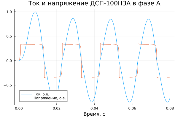
.The waveform has the expected shape; additionally, these two signals can be represented as a volt-ampere characteristic (VAC).:
plot(IarcA_pu, VarcA_pu;
    label = :none, title = "VAH CHIPBOARD-100NZA",
    xlabel = "Current Ia, O.E.", ylabel = "Voltage Va, O.E.")
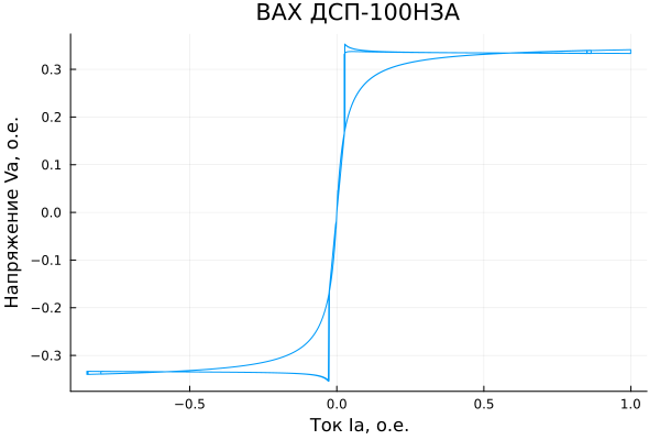
The VAC of the furnace arc also has the expected shape. Therefore, the model constructed according to the description from the publication is correct. Let's proceed to the analysis of harmonic distortions of current and voltage.
Harmonic analysis
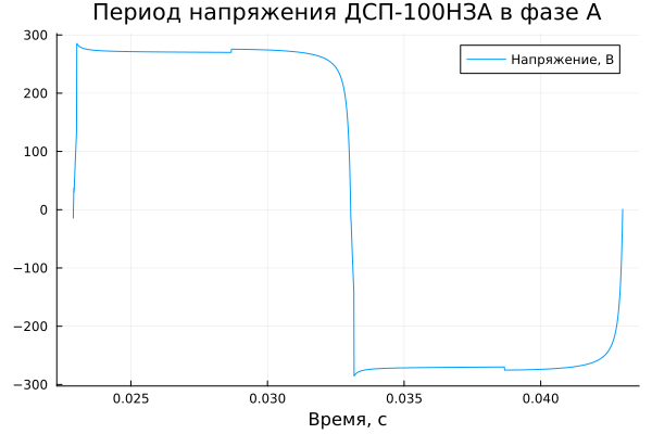
To analyze harmonics in static mode, it is enough to take one period of the signal. This will be the furnace arc voltage signal in phase A in the next interval.:
gr()
int = 2290:4301
plot(t[int],  VarcA[int];
    label = "Voltage, V",
    title = "DSP-100NZA voltage period in phase A",
    xlabel = "Time, from")
We get the signal and time vectors for this interval:
signal = VarcA[int]; t = t[int];
Using the functions from the Julia script, we will get data on the amplitudes and phases of the harmonic components of a given section of the signal.:
# Analyzing harmonics
results = analyze_harmonics(signal, fs, fc)

n, A, ph = get_harmonics_data(results)

# We display the results
println("Harmonic | Amplitude | Phase (degree)")
println("----------------------------------")
for (n, A, ph) in zip(n, A, ph)
    round(A, digits=3)!=0.0 ? println(lpad(n, 9), " | ", lpad(round(A, digits=3), 9), " | ", round((ph)*180/pi, digits=3)) : nothing
end
Using the following function, we will separate the distortion data for the harmonics of the forward, reverse and triple sequences.:
harm, harm2, harm3 = get_sequences(results, n);
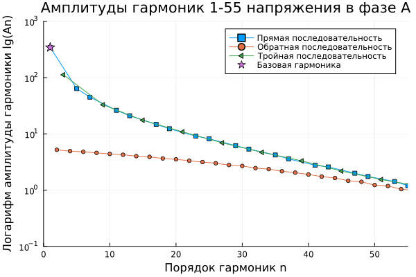
The amplitudes of each of the harmonics highlighted in the sequence can also be conveniently represented on the graph in logarithmic axes.:
gr()
plot( yaxis = :log, xlims=[0,55],ylims=[1e-1,1e3], title = "Amplitudes of harmonics 1-55 of voltage in phase A", xlabel="Harmonic order n", ylabel = "Logarithm of harmonic amplitude lg(An)")
plot!(harm[1], harm[2];
        markershape = :square, markersize=3, label = "The direct sequence")
plot!(harm2[1], harm2[2];
        markershape = :circle, markersize=3, label = "Reverse sequence")
plot!(harm3[1], harm3[2];
        markershape = :ltriangle, markersize=5, label = "The triple sequence")
scatter!([harm[1][1]], [harm[2][1]];
        markershape = :star, markersize=7, label = "The basic harmonic")
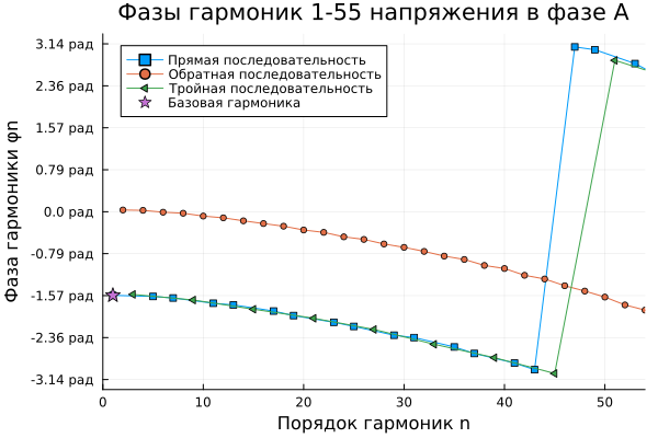
A similar graph can be presented for the phases of each of the harmonics in the sequences.:
gr()
y = range(-π, π, length=9)
plot(xlims=[0,54], yticks = (y, ["$(round(yi, digits=2)) glad" for yi in y]), title = "Harmonic phases 1-55 voltage in phase A", xlabel="Harmonic order n", ylabel = "Harmonic phase φn")
plot!(harm[1], harm[3];
        markershape = :square, markersize=3, label = "The direct sequence")
plot!(harm2[1], harm2[3];
        markershape = :circle, markersize=3, label = "Reverse sequence")
plot!(harm3[1], harm3[3];
        markershape = :ltriangle, markersize=5, label = "The triple sequence")
scatter!([harm[1][1]], [harm[3][1]];
        markershape = :star, markersize=7, label = "The basic harmonic")
Levels of total harmonic distortion
The total levels of harmonic distortion that can be used to correlate with electrical energy quality standards according to GOST 32144-2013 are determined by the Euclidean norm formula.:
Let's calculate the levels of harmonic voltage distortion - the total for all harmonics and for individual sequences.
THD_V = norm(vcat(harm[2][2:end], harm2[2], harm3[2]))/harm[2][1]*100;
THD_V0 = norm(harm[2][2:end])/harm[2][1]*100;
THD_V2 = norm(harm2[2])/harm[2][1]*100;
THD_V3 = norm(harm3[2])/harm[2][1]*100;

println("Total harmonic distortion factor of voltage: ", round(THD_V, digits=2), "%.\Without it, by sequence:")
println("- direct: ", round(THD_V0, digits=2), "%,")
println("- reverse: ", round(THD_V2, digits=2), "%,")
println("- triple: ", round(THD_V3, digits=2), "%.")
Calculate the harmonic distortion for the current:
results_I = analyze_harmonics(IarcA, fs, fc);
n_I, A_I, ph_I = get_harmonics_data(results_I);
THD_I = norm(A_I[2:end])/A_I[1]*100

println("Total harmonic distortion of the current: ", round(THD_I, digits=2), "%.")
Conclusion
In this project, a static model of the DSP-100NZA arc steelmaking furnace was developed, modeling was carried out, current and voltage waveforms and harmonic analysis data were obtained. The obtained materials will form the basis for further examples related to mode modeling, chipboard control, and improving the quality of electricity.
Literature
Chernenko, A. N. Dynamic furnace arc model in Matlab (Simulink) / A. N. Chernenko, V. V. Vakhnina, S. G. Martynova // Vector of Science of Tolyatti State University. – 2015. – № 2-1(32-1). – Pp. 58-64. – [EDN TYKPDV] (https://www.elibrary.ru/item.asp?id=23675896 ).