Recirculating drive with differential cylinders
This example demonstrates the operation of a two-way hydraulic drive with differential cylinders. The pump outlet is connected to the cylinder B, while the cylinder A is connected to the pump and then to the hydraulic tank using a three-way distribution valve controlled by a sinusoidal signal.
When cylinder A is connected to the pump, the pressure in both cylinders equalizes. However, due to the larger effective area of the piston in the cylinder A, the force on its side exceeds the force in the cylinder B, which leads to the extension of the rod. When cylinder A is connected to the hydraulic tank, the rod begins to retract.
General view of the model
The subsystem of mechanical load
The external load on the cylinder rod is represented by a conventional spring-damper subsystem. The movement of the rod leads to a mass displacement of 50 kg.
.png)
Subsystem of external conditions
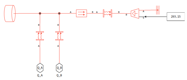
The heat from the cylinder is dissipated in two ways: through the cylinder walls into the air and through the hydraulic fluid, which carries the heat into the main line. On the right side of this model is a radiator that maintains the temperature of the liquid at 20 degrees Celsius.
The thermal mass (5 kg) in the diagram can simulate the effect of heat accumulation in the cylinder body and part of the hydraulic system, which cools and heats up more slowly, smoothing out sudden temperature fluctuations.
.png)
Simulation results
engee.addpath(@__DIR__)
model = engee.open("reciprocal-actuator-with-differential-cylinders.engee");
data = engee.run(model);
Here are some graphs describing the operation of this system.:
plot(data["pistonPosition"].time, data["pistonPosition"].value,
     title="Cylinder stem position (m)", legend=false,
     lw=2, titlefont=font(11), size=(800,400))
valve_area_PA = data["3-way valve (TJ).orifice_pa.orifice_area"];
valve_area_AT = data["3-way valve (TJ).oriifice_at.oriifice_area"];
plot(valve_area_PA.time, 1000 .* [valve_area_PA.value valve_area_AT.value],
     label=["Hole P-A" "Hole A-T"],
     title="Opening area of the three-way valve (mm)", lw=2, titlefont=font(11), size=(800,400))
force_A = data["Double-acting drive (TJ).chamber_a.F"];
force_B = data["Double-acting drive (TJ).chamber_b.F"];
plot(force_A.time, [force_A.value force_B.value],
     label=["Side A" "Side B"],
     title="Forces acting on each side of the drive (H)", lw=2, titlefont=font(11), size=(800,400))
The graphs show:
-
Three-way valve opening area
-
Forces acting on each side of the drive during the reciprocating motion.
Conclusion
The scope of application of such drives is very wide. They are used wherever a long stroke is required in a limited space, and are found in excavators, loaders, bulldozers, combines and tractors, presses and machine tools, as electrohydrostatic drives in aviation and astronautics, in jacks and cranes.
This example shows how to calculate the operation of a hydraulic drive to avoid errors and optimize system performance.