Bipolar transistor in low-voltage mode
In this example, we use an equivalent substitution circuit to evaluate the performance of a bipolar transistor. The transistor is switched on according to a common-emitter circuit and operates in a low-signal (linear) mode.
We will use the Mask to create our own transistor block.
Description of the model
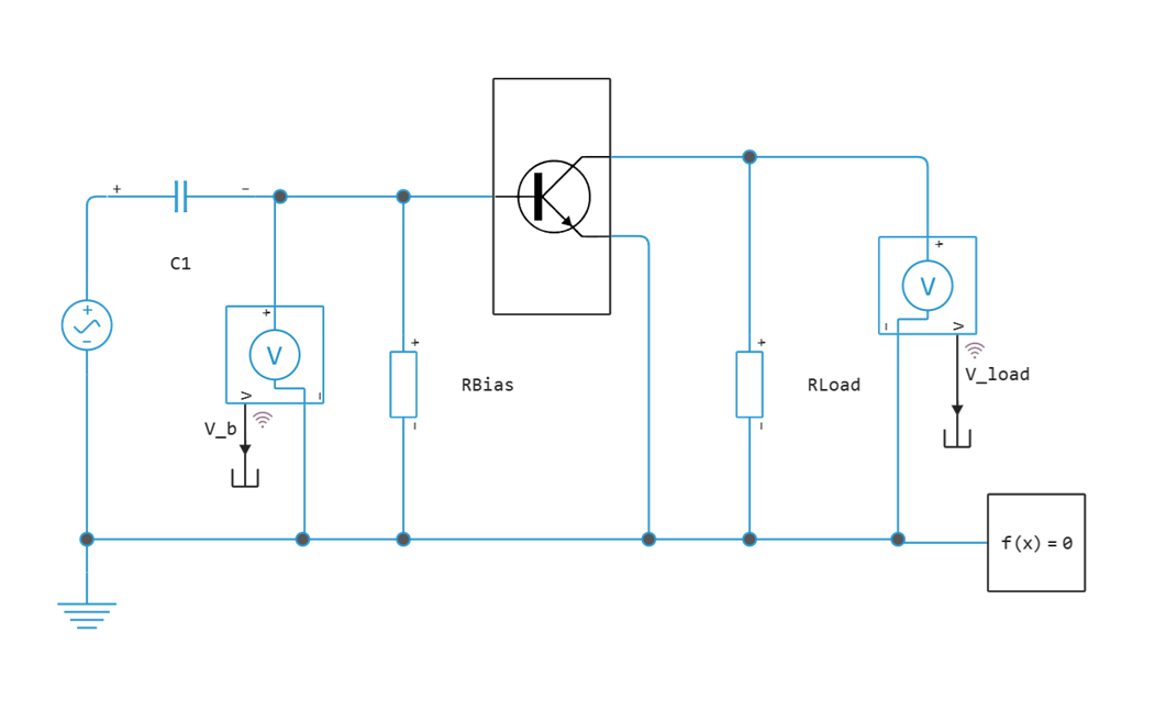
The transistor is represented by an equivalent circuit with h-parameters:
- input resistance,
- output conductivity,
- current transfer coefficient,
- voltage feedback coefficient.
The parameters are set for the BC107-B transistor:
h_ie = 3000.0;
h_oe = 60e-6;
h_fe = 300.0;
h_re = 3e-4;
There are two resistors in the model:
- Rbias (47 kOhm) is a bias resistor. Sets the nominal operating point.
- Rload (470 ohms) - load resistor.
The gain is approximately determined by the expression:
The separation capacitor C1 (1 UF) is selected so that its resistance at a frequency of 1 kHz is negligible compared to the input resistance . The peak output voltage should be .
Simulation of the model
engee.addpath(@__DIR__)
if "SmallSignalBipolarTransistor" in [m.name for m in engee.get_all_models()]
    m = engee.open( "SmallSignalBipolarTransistor" ) # loading the model
else
    m = engee.load( "SmallSignalBipolarTransistor.engee" )
end
results = engee.run(m, verbose=true)
t = results["V_b"].time;            # Time
V_b  = results["V_b"].value;        # Offset voltage
V_load  = results["V_load"].value;  # Load voltage
plot(t, V_b, title="Transistor voltage", xlabel="Time, c", ylabel="Voltage, V", w = 2, label="Base")
plot!(t, V_load, xlabel="Time, c", ylabel="Voltage, V", w = 2, label="Collector")
The model shows how more complex elements, in this case a transistor, can be built from blocks of the Physical Modeling/Fundamental library and hidden under a Mask.