The pipeline between the two tanks
In this example, we will show how to calculate the flow capacity of a pipe when an incompressible liquid passes through it under excessive pressure.
Description of the model
The model of this simple pipeline system contains two reservoirs (a block Reservoir), the first of which has an overpressure of 50,000 Pa relative to the second. The basic pressure value in both cases is atmospheric pressure (101,325 Pa), but it does not play a special role here, including because an incompressible liquid flows through the pipe.
Pipe (Pipe (IL)) is characterized by a length of 10 meters and a diameter of 0.2 m (cross -sectional area pi*(0.1^2) м2).
From the "service" blocks, the model contains a block for setting fluid parameters Isothermal Liquid Properties (IL) and the block Solver Configuration – both have default settings.
Model Execution
Let's launch this model:
modelName = "reservoirs_pipe"

if modelName ∉ [m.name for m in engee.get_all_models()] engee.load( "$(@__DIR__)/$modelName.engee"); end;

data = engee.run( modelName )
Let's show the fluid flow rate found by the model through this pipe.:
data["Expenditure"].value[end]
So, the throughput of a 0.2 m diameter pipe with a length of 10 m when water is pumped into it with an excess pressure of 0.05 MPa is 269.9 kg/s.
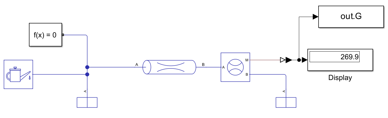
Comparison with the Simulink model
A similar model assembled in the Simulink environment shows the same result: the flow rate through the pipe is 269.9 kg/s.
.png)
If desired, you can run the attached model and double-check the result.
using MATLAB

demoroot = @__DIR__
mat"start_simulink"
mat"p = $demoroot; addpath(p);"
mat"p = '/user/start/examples/helper_units'; addpath(p);"

mat"simout = sim('reservoirs_pipe_2023a.slx');"
mat"disp( simout.G.Data(end) )"
Conclusion
We created a very simple model and solved the problem of calculating the flow of water through a pipe under certain conditions. The results exactly matched the model created in Simulink.