Calculation of the mass flow rate during the flow of liquid through pipes of various shapes of cross sections
This example demonstrates the use of the Laminar Leakage block of the Isothermal Fluid library.
This block simulates laminar flow through sections of various geometries in an isothermal fluid network.
The example considers sections such as a circle, rectangle, ellipse, and equilateral triangle.
The cross-sectional areas of the pipes are equal to each other.
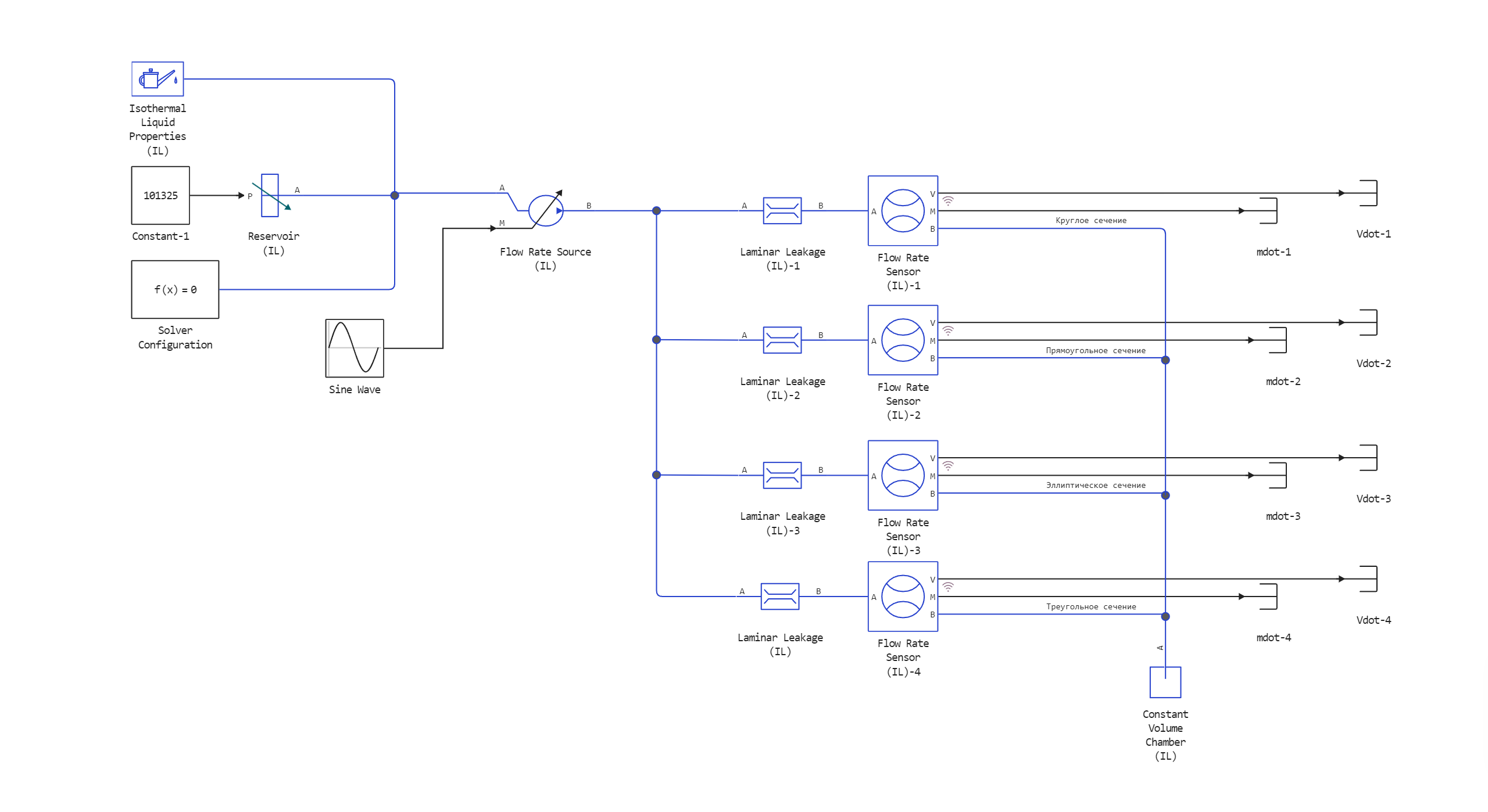
Model diagram:
Defining a function to load and run the model:
function start_model_engee()
    try
        engee.close("npn_transistor", force=true) # closing the model
        catch err # if there is no model to close and engee.close() is not executed, it will be loaded after catch.
            m = engee.load("$(@__DIR__)/laminar_leakages.engee") # loading the model
        end;

    try
        engee.run(m, verbose=true) # launching the model
        catch err # if the model is not loaded and engee.run() is not executed, the bottom two lines after catch will be executed.
            m = engee.load("$(@__DIR__)/laminar_leakages.engee") # loading the model
            engee.run(m, verbose=true) # launching the model
        end
end
Loading, running the model, and recording the results
Running the simulation
try
    start_model_engee() # running the simulation using the special function implemented above
    catch err
    end;
Extracting mass expense data from the simout variable:
sleep(5)
result = simout;
res = collect(result)
Recording the results of the model in separate variables:
circular_flowrate = collect(res[3])
rectangular_flowrate = collect(res[2])
elliptical_flowrate = collect(res[4])
triangular_flowrate = collect(res[1]);
Visualization of simulation results
using Plots
plot(circular_flowrate[:,1], circular_flowrate[:,2], label="Round section", lw = 3, title="Mass flow through sections", xlabel="Time, from", ylabel="Mass flow rate, kg/s", legend=:bottomright)
plot!(rectangular_flowrate[:,1], rectangular_flowrate[:,2], label="Rectangular cross section", lw = 3)
plot!(elliptical_flowrate[:,1], elliptical_flowrate[:,2], label="Elliptical section", lw = 3)
plot!(triangular_flowrate[:,1], triangular_flowrate[:,2], label="Triangular section", lw = 3)
Conclusion:
This example demonstrates the simulation of a hydraulic network with Laminate Leakage blocks, each of which is a pipe with specified geometric cross-sectional parameters. Analyzing the simulation results, one can see the difference in the mass flow rates of these pipes depending on the shape of the cross-section of the same area.